Fusion Of Flow-based Model And Diffusion Model ~DiffFlow~

3 main points
✔️ Diffusion Normalizing Flow (DiffFlow) extends flow-based and diffusion models and combines the advantages of both methods
✔️ DiffFlow improves model representativeness by relaxing the total monojectivity of the function in the flow-based model and improves sampling efficiency over the diffusion model
✔️ DiffFlow also generates complex fine features of the distribution that could not be modeled with flow-based or diffusion models

Diffusion Normalizing Flow
written by Qinsheng Zhang, Yongxin Chen
(Submitted on 14 Oct 2021)
Comments: Neurips 2021
Subjects: Machine Learning (cs.LG)

code：  

 

The images used in this article are from the paper, the introductory slides, or were created based on them.

first of all

A deep learning model that learns a data distribution and artificially generates unknown data is called a deep generative model. The deep generative model learns a neural network that generates data $\mathbb{x}$ from a latent variable $\mathbb{z}$.

Among them, there are those in which the dimensions of the latent variable and the data are equal, and in these models, the process of generating data from the latent variable can be treated as a trajectory in the same space. When this trajectory is determined deterministically, it is called a flow-based model, and when it is determined stochastically, it is called a diffusion model.

Flow-based models generate data by applying sequential transformations to latent variables using functions. The problem is that the expressive power of the model is limited by the restriction that this function must be reversible.

On the other hand, the diffusion model consists of a diffusion process that successively adds noise to the data to reduce it to a simple latent variable and an inverse process that recovers the data by gradually removing the noise. The inverse process has the disadvantage that the noise addition in the diffusion process must be slow enough to generate high-quality samples, and the model training is time-consuming. The nature of adding noise independently from the data distribution also makes it difficult to capture detailed features within the distribution.

The Diffusion Normalizing Flow (DiffFlow) method introduced in this paper combines the best of the two methods to generate data based on the drawbacks of the flow-based model and the diffusion model described above. In the next section, we will briefly introduce the flow-based model and the diffusion model, and then give an overview of DiffFlow.

What is a flow-based model (normalized flow)?

In the flow-based model (normalized flow), the aforementioned trajectory in space is modeled by the following differential equation

Here $\mathbb{x}(0)$ represents the starting point, the data, and $\mathbb{x}(T)$ represents the endpoint, the latent variable $z$. The $T$ denotes the time step to the time $T$ when it is transformed into a latent variable.

Here, assuming continuous time, the following relation is derived

In addition, if we assume discrete time, the following relation is derived. In this case, the mapping from data to latent variables is a composite function of all single-shot functions $F=F_N \circ F_{N-1} ... F_{2} \circ F_{1}$.

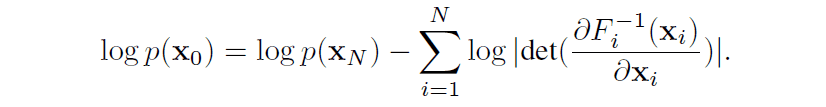
The flow-based model is characterized by its ability to calculate the data likelihood directly, as expressed in the above equation.

What is a diffusion model?

The trajectory in space in the diffusion model is modeled by stochastic differential equations. The diffusion process from data to latent variables is represented by the following relation In the equation $\mathbb{f}$ is a function that outputs a vector and is called the drift term. And $g$ is a scalar function and is called diffusion coefficient.

The inverse process from latent variable to data can also be expressed by the following relationship

It is known that the function $\mathbb{s}$ in the inverse process coincides with the score function $\nabla \log(p_F)$ of the distribution $p_F$ on the trajectory in the diffusion process, and the distribution $p_B$ on the trajectory in the inverse process coincides with $p_F$ under the condition that the latent variables in both processes share the same distribution The following is an example.

In the diffusion model, $\mathbb{s}$ approximated by a neural network is trained to minimize the difference between the distributions of $p_F$ and $p_B$, and data are generated using sampling in the inverse process. The KL divergence is mainly used as a measure of the difference in this distribution.

Under discrete-time conditions, $p_F$ and $p_B$ can be expressed as follows, respectively. It may be easier to grasp the image of the diffusion process and inverse process.

In the diffusion model, the data likelihood cannot be obtained directly, so the lower bound of the log-likelihood is calculated.

DiffFlow

The Diffusion Normalizing Flow (DiffFlow) proposed in this paper proposes a model that is located between the normalizing flow and the diffusion model. The two-way process between data and latent variables is illustrated in the following figures for normalized flow, diffusion model, and DiffFlow.

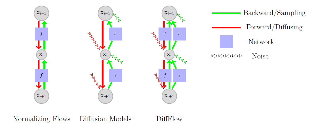
The major difference is that the function $f$, which has been represented only as a simple linear function in the diffusion process, can be approximated and learned by a neural network, and noise is introduced in the part of the function $f$ that did not exist in the normalized flow.

The flow-based model uses only invertible functions, which guarantees that the data will be recovered, but does not guarantee that the Gaussian noise will be reached in the end. On the other hand, the diffusion model adds noise that is independent of the data, so it can reach the Gaussian noise in only one step by completely ignoring the data. However, this does not generate data because the inverse process cannot be learned.

By adding a new learnable function $f$ in the process of transforming data to latent variables, DiffFlow is considered to provide a sufficient supervised signal for learning in the inverse process of sampling the data.

In the implementation, we use the following equations (upper: diffusion process, lower: inverse process) as the diffusion process and inverse process in discrete time.

In the equation, $\delta$ represents the noise sampled from the multivariate standard normal distribution and $\Delta t$ represents the discretized time step.

The loss function is derived from the KL divergence for two distributions, $p_F$ for the diffusion process and $p_B$ for the inverse process, and DiffFlow trains the function $f,s$ to minimize this loss function.

DiffFlow takes measures against memory consumption when computing gradients and changes the interval when discretizing time steps. See the original paper for details.

Now that you have a rough idea of how DiffFlow works, let's look at the results of data generated using this method.

Diffusion Processes in Artificial Data

First, let's look at the results of visualizing the diffusion process in artificial data.

The figure below illustrates the transformation from data to latent variables in DiffFlow (this method), DDPM (diffusion model), and FFJORD (flow-based model). The results are shown when dealing with different rings of data on the left and right.

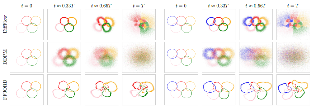
In FFJORD, which is a flow-based model, the ring shape remains after conversion to latent variables, and the points are not scattered over the entire space. On the other hand, DDPM, which is a diffusion model, finally obtains latent variables that are scattered over the entire space, but each mode (the color-coded rings in the figure) is represented as a mixture of modes.

In DiffFlow, the distribution of the latent variable over the entire space is obtained while maintaining the characteristics of the ring, which is a good combination of the flow-based model and the diffusion model.

Generating artificial data in the inverse process

Next, we show the results of sampling images from latent variables using the inverse process concerning the artificial data.

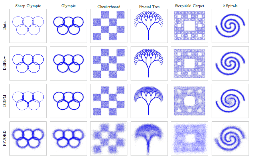
All of the models can generate a distribution that captures the original data distribution, but only DiffFlow can capture the detailed shape of the distribution. This result suggests that DiffFlow may be able to successfully generate data on complex datasets with sharper boundaries.

in conclusion

I was surprised that DiffFlow was able to reproduce and generate quite a lot of fine details. VAE and GAN are familiar as deep generative models now, but flow-based models and diffusion models are likely to attract more attention in the future.

It is discussed in the paper that DiffFlow has a slower computation time than conventional diffusion models, and it still seems to be inferior to other generative models when it is actually applied to the generation of high-dimensional data such as images.

• 
• 
• 

Categories related to this article

• Generative Model
• Flow-based Model
• Diffusion Model
• Diffusion Model