GT-GAN, Which Enables Time Series Data Synthesis By Unifying Even Missing Data Columns
3 main points
✔️ In time series data synthesis, it has traditionally been difficult to handle regular data and irregular data with missing data in a single generative model.
✔️ GT-GAN is a GAN, auto-encoder, neural ordinary differential equation, neural control differential equation, and continuous-time flow process GT-GAN is a synthesis of three data flows combining models.
✔️ irregular data is complemented through ordinary differential equations in the decoder, backpropagation to the generator from hidden vector data, and unified data generation with regular data as well.
AutoFormer: Searching Transformers for Visual Recognition
written by Jinsung Jeon, Jeonghak Kim, Haryong Song, Seunghyeon Cho, Noseong Park
(Submitted on 5 Oct 2022 (v1), last revised 11 Oct 2022 (this version, v3))
Comments: NeurIPs 2022
Subjects: Machine Learning (cs.LG); Artificial Intelligence (cs.AI)
code:
The images used in this article are from the paper, the introductory slides, or were created based on them.
summary
This is a NeurIPS 2022 accepted paper. Time series synthesis is one of the key research topics in the field of deep learning and can be used to augment data. Time series data can be broadly classified into two types: regular and irregular (series are flawed). However, for both types, there are no existing generative models that show good performance without model modification. Therefore, we propose a generic model that can synthesize regular and irregular time series data. To the best of our knowledge, this paper is the first to design a generic model for one of the most challenging settings of time series synthesis. For this purpose, we have designed a method based on generative adversarial networks and carefully integrated many related techniques ranging from neural ordinary/controlled differential equations to continuous-time flow processes into a single framework. This method outperforms all existing methods.
Introduction
Because real-world time series data are frequently unbalanced and/or inadequate, synthesizing time series data has become one of the most important of the many tasks associated with time series. However, because regular and irregular time series data have different characteristics, different model designs have been employed for both. Therefore, existing time series synthesis research focuses on either regular or irregular time series synthesis [Yoon et al. 2019, Alaa et al. 2021]. To the best of our knowledge, there are no existing methods that work well with both types.
A regular time series means regularly sampled observations with no missing values, while an irregular time series means that some observations are missing from time to time. Irregular time series are much more difficult to process than regular time series. For example, it is known that the performance of neural networks improves after the time series data is transformed to its frequency domain, i.e., Fourier transform, and several time series generation models use this approach [Alaa et al., 2021]. However, it is not easy to observe predetermined frequencies from highly irregular time series [Kidger et al., 2019]. Here, continuous-time models [Chen et al. 2018, Kidger et al. 2020, Brouwer et al. 2019] have shown good performance in handling both regular and irregular time series. Based on them, this paper proposes a generic model that can synthesize both time series types without model modifications.
To achieve its goals, the method uses a variety of techniques ranging from generative adversarial networks (GANs [Goodfellow et al., 2014]) and autoencoders (AEs) to neural ordinary differential equations (NODEs [Chen et al., 2018]), neural control differential equations (NCDEs [ Kidger et al., 2020]), to continuous time flow processes (CTFPs [Deng et al., 2020]), we design advanced models using diverse techniques. This reflects the difficulty of the problem.
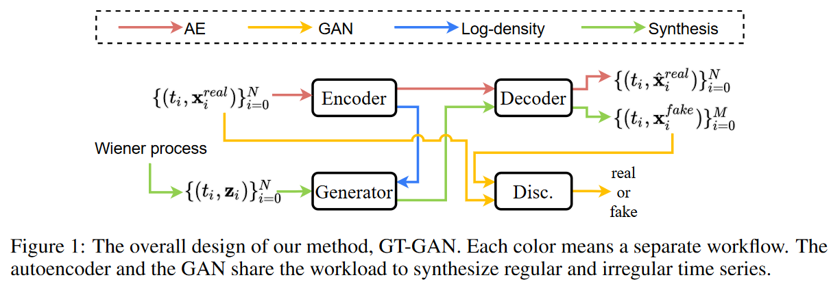
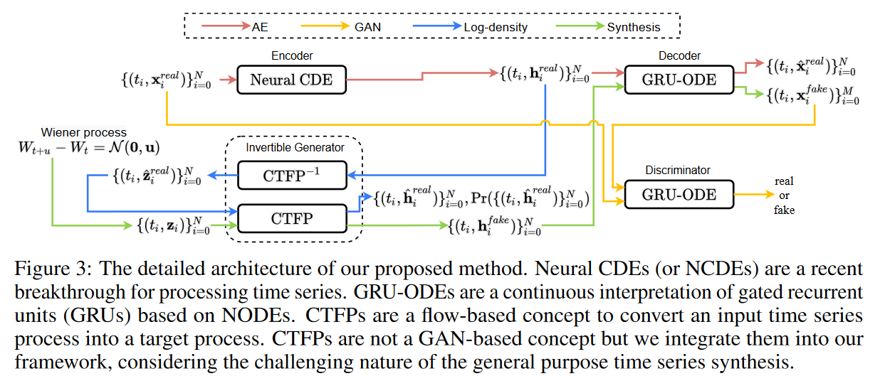
Fig. 1 shows the overall design of the proposed method. The key point of the proposed method is that it combines adversarial learning of GAN and exact maximum likelihood learning of CTFP in one framework. However, exact maximum likelihood learning is only applicable to reversible mapping functions where the input and output sizes are the same. Therefore, in this paper, we design an invertible generator and employ an autoencoder where the GAN performs adversarial learning in its hidden space. Namely,
i) the hidden vector size of the encoder is the same as the noisy vector of the generator, and
ii) The generator generates a set of false hidden vectors and
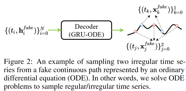
iii) The decoder converts the set into a false continuous path (see Fig. 2)
iv) The discriminator reads the sampled false samples and provides feedback.
We emphasize that in the third step, the decoder creates a false continuous path. Thus, any regular/irregular time series samples can be sampled from the false path, demonstrating the flexibility of this method.
Experiments were conducted on four datasets and seven baselines. Both regular and irregular time series were tested. The method performed better than the other baselines in both environments.
The contributions of this methodology can be summarized as follows
1. design models based on various state-of-the-art deep learning techniques. The method is capable of processing all types of time series data, from regular to irregular, without model modification.
2. Prove the effectiveness of the proposed model through experimental results and visualization.
3. since our task is one of the most challenging in time series synthesis, the architecture of the proposed model is carefully designed.
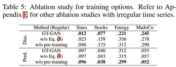
4. Isolation studies have shown that the proposed model does not work well if any part is missing.
Proposed Method
Because time series synthesis is a difficult task, the proposed design is much more complex than other baselines.
Overall workflow
First, the overall workflow consists of several different data paths (and several different learning methods based on the data paths), as described below.
1. auto encoder path
Given a time-series sample, the encoder generates a set of hidden vectors. The decoder recovers a continuous path, which increases the flexibility of the proposed method. Sampling from this path. The encoder and decoder are trained using standard autoencoder (AE) loss to match the continuous path and sampling values for all sampling points.
2. hostile channel
Given a noise vector, the generator generates a set of false hidden vectors. The decoder recovers false continuous paths from the false hidden vectors. For the synthesis of irregular time series, tj is sampled at [0, T ]. The generator, decoder, and discriminator are trained with standard adversarial loss.
Logarithmic density path
Given a set of hidden vectors for the time series samples, the inverse pass of the generator regenerates the noise vectors. During the forward pass, inspired by Grover et al. [2018] and Deng et al. [2020], the negative log probability for all sampling time points i is computed with the variable change theorem and learned by minimizing it.
In particular, note that the dimension of the autoencoder's hidden space is the same as the dimension of the generator's potential input space, i.e., dim(h) = dim(z). This is necessary for exact likelihood learning in the generator to estimate the exact likelihood, the variable change theorem requires that the magnitudes of the input and output be the same. In addition to this, the task of synthesizing the false time series is shared by integrating the autoencoder and the generator into a single framework. That is, the generator synthesizes the false hidden vectors and the decoder regenerates the human-readable false time series from them.
Auto Encoder
Encoder
A typical NCDE is considered a continuous analog of a recurrent neural network (RNN) and is defined as follows
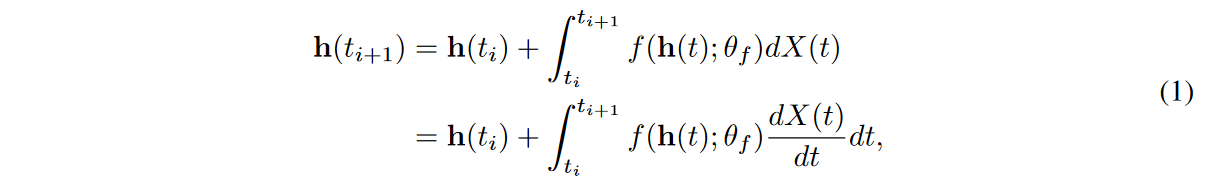
where X(t) is a continuous path created by the interpolation algorithm from the raw discrete time series samples {(ti,xreal i ) }N i=0, where X(ti ) = ( ti, xreal i ) for all i, and for other unobserved time points the interpolation algorithm fills in values Note that NCDE continues to read the time derivative of X(t). In this case, we collect {hreal i }N i=0 as follows

where hreal 0 = FCdim (x)→dim(h)( xreal 0 ) and FCinput_size→output_size have fully connected layers with specific input and output sizes. Thus, an input time series {(ti,xreal i ) }N i=0 is represented by a set of hidden vectors {(ti, hreal i ) }N i=0. NCDEs are continuous analogs of RNNs, indicating that they are most suitable for processing irregular time series [Kidger et al., 2020].
Decoder
The decoder for this method of recreating time series from hidden representations is based on GRU-ODE [Brouwer et al., 2019] and is defined as follows
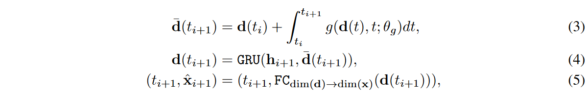
where d( t0) = FCdim (h) → dim(d) (h0) and hi means the i-th real or false hidden vector, i.e., hreal i or hfake i. Recall that in Fig. 3, the decoder is involved in both the autoencoding and the synthesis process; GRU-ODEs use a technique called neural ordinary differential equations (NODEs) to interpret GRUs continuously.
In particular, gated recurrent units (GRUs) in equation (4) are called jumps, which are known to be effective for time series processing with NODEs [Brouwer et al., 2019, Jia and Benson, 2019]. For all training time series samples, we train the encoder-decoder using the standard reconstruction loss between xreal i and ˆ xreal i for all i.
generic adversary network
Generator
In standard GANs, generators typically generate false samples by reading noisy vectors, whereas the generator in this method generates false time series samples by reading continuous paths (or time series) sampled from the Wiener process. This generative concept is known as a continuous time flow process (CTFP [Deng et al., 2020]). The input to the generative process of this method is a random path sampled from the Wiener process, which is represented by a time series of latent vectors of the path, and the output is a hidden vector path, also represented by a time series of hidden vectors.
Thus, the generator can be written as follows

where τ is the virtual time variable of the integration problem and ti is the real physical time contained in the time series sample {(ti,xreal i ) }M i=0. We emphasize that this design corresponds to the NODE model extended by ai ( t).
Thanks to the reversible nature of NODE, the exact log density of hreal i, i.e., the probability that hreal i is generated by the generator, can be calculated as follows using the change of variable theorem and Hutchinson's stochastic trace estimator [Graswohl et al. 2019, Deng et al, 2020].
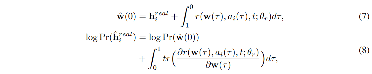
Equation (7) corresponds to "CTFP-1" in Fig. 3, while Equations (6) and (8) correspond to "CTFP". Note that in equation (7), the integration time is reversed to solve the inverse mode integration problem. So, we minimize the negative logarithmic density for each ti and train the generators in two different learning paradigms: i) adversarial learning for the discriminator and ii) maximum likelihood estimator (MLE) learning using the logarithmic density.
Discriminator
Based on GRU-ODE technology, the discriminator is designed as follows
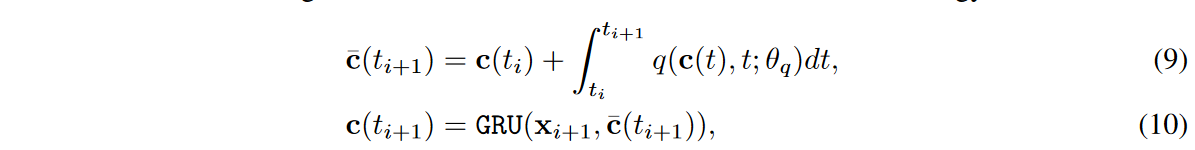
where c( t0) = FCdim (x) → dim(c) (x0), xi means the i-th time series value, i.e., xreal i or xfake i. The ODE function q has the same architecture as g but has its parameter θq. We then compute the real or fake classification y = σ(FCdim (c) → 2 (c( tN ))), where σ is the softmax activation.
Learning Methods
To train the encoder-decoder, we use the average squared restoration loss, i.e., the average of ‖xreal i -ˆ xreal i ‖22 for all i. The standard GAN losses are then used to train the generators and discriminators. Preliminary experiments show that the original GAN losses are suitable for the task of this method. Therefore, we use standard GAN losses instead of other variants such as WGAN-GP [Gulrajani et al. 2017]. We train the model in the following order.
1. pre-train the encoder-decoder network for reconfiguration loss for KAE iterations.
2. In the KJOINT iteration, after the above pre-training, start joint training of all networks in the following order: i) train the encoder-decoder network with reconstruction loss, ii) train the discriminator-generator network with GAN loss, iii) train the decoders that improve the classifier classification output with discriminator loss MLE training at each PMLEiteration, as it was found that too frequent MLE training can lead to mode collapse.
In particular, the 2-ii step of training the decoder to help the discriminator is one additional point where the autoencoder and GAN are integrated into a single framework. In other words, the generator needs to fool both the decoder and the discriminator.
The well-posedness of NCDE and GRU-ODE has already been proved in Lyons et al. [2007, Theorem 1.3] and Brouwer et al. [2019] under the mild condition of Lipschitz continuity. This paper shows that the NCDE layer of our method is also a good setting problem: almost all activation functions such as ReLU, Leaky ReLU, SoftPlus, Tanh, Sigmoid, ArcTan, Softsign, etc. have a Lipschitz constant of 1, and there is no drop-out, batch normalization, or other Other common neural network layers, such as pooling methods, have explicit values for the Lipschitz constant. Therefore, the Lipschitz continuity of the ODE/CDE function can be satisfied in the case of this method. In other words, it is a well-solved learning problem. As a result, our learning algorithm solves a good-set problem and its learning process is practically stable.
experimental evaluation
test environment
Data Set
In this paper, we experimented on two simulated datasets and two real-world datasets; Sines has five features, each independently created at a different frequency and phase. For each feature, i ∈ {1, 5}, xi(t) = sin(2πfit + θi), where fi ∼ U [0, 1] and θi ∼ U [-π, π]; MuJoCo is multivariate physics simulation time series data with 14 features; Stocks is Google stock price data from 2004 to 2019 Stocks is Google's stock price data from 2004 to 2019. Each observation represents one day and has 6 features; Energy is the UCI appliance energy forecast dataset with 28 values. To create a challenging random environment, each time series sample {(ti, xreal i )}N i=0 to 30, 50, and 70% of the observations are randomly dropped. Dropping random values is mainly used in the literature to create irregular time series environments [Kidger et al. 2019, Xu and Xie, 2020, Huang et al. 2020b, Tang et al. 2020, Zhang et al. 2021, Jhin et al. ., 2021, Deng et al., 2021]. Thus, we experiment in both regular and non-regular environments.
Baseline
For experiments with regular time series, the following baselines are considered: TimeGAN, RCGAN, C-RNN-GAN, WaveGAN, WaveNet, T-Forcing, and P-Forcing. For the irregular experiments, we excluded WaveGAN and WaveNet, which cannot handle irregular time series, and the other baselines were redesigned by replacing their GRUs with GRU-4t and GRU-Decay (GRU-D) [Che et al, 2018].GRU-4t and GRU-D are irregular time series data; GRU-4t additionally uses time differences between observations as input; GRU-D is a modification of GRU-4t to learn exponential decay between observations: TimeGAN-4t, RCGAN-4t, C-RNN-GAN-4t, T-Forcing-4t, P-Forcing-4t (resp. TimeGAN-D, RCGAN-D, C-RNN-GAN-D, T-Forcing-D, P-Forcing-Decay) were modified in GRU-4t (resp. GRU-D) to be able to handle irregular data. In addition, many advanced methods are used in our ablation studies, such as NODE, VAE, and flow models. Since the proposed method has these advanced methods as internal subparts, we dare to leave them in the ablation study.
Evaluation Indicators
For quantitative evaluation of the synthesized data, we use the discriminative and predictive scores used in TimeGAN [Yoon et al., 2019]. The discriminative score measures the similarity between the original and synthetic data. After training a model to classify the original and synthesized data using a neural network, it tests whether the original and synthesized data are well classified. The Discrimination Score is |Accuracy-0.5|, and a low score indicates that the original and synthetic data are similar because classification is difficult. The prediction score measures the validity of the synthetic data using the train-synthesis-and-test-real (TSTR) method. After training a model to predict the next step using the synthesized data, we calculate the mean absolute error (MAE) between the predictions and the grand-truth values of the test data; if the MAE is small, we determine that the model trained on the synthesized data is similar to the original data. For qualitative evaluation, we visualize the synthesized data with the original data. There are two methods for visualization. One is to use t-SNE [Van der Maaten and Hinton, 2008] to project the original and synthetic data in a two-dimensional space. The other is to draw the distribution of the data using kernel density estimation.
experimental results
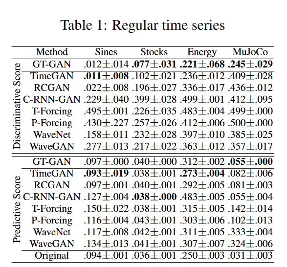
Normal time series synthesis
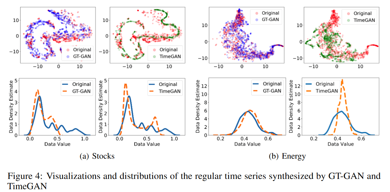
In Table 1, we list the results of the usual time series synthesis, and GT-GAN performs better than the traditional state-of-the-art model, TimeGAN, in most cases. as shown in the first row of Fig. 4, GT-GAN covers the original data domain better than TimeGAN, and the results of the time series synthesis are shown in the second row of Fig. 5. as shown in the first row of Fig. 4. The second row of Fig. 4 shows the distribution of false data generated by GT-GAN and TimeGAN; the distribution of synthetic data in GT-GAN is closer to the distribution of the original data than in TimeGAN, indicating that GT-GAN's explicit likelihood learning is more effective than TimeGAN's implicit likelihood learning.
Irregular time series synthesis
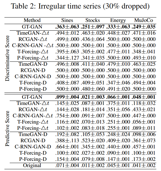
Tables 2, 3, and 4 lists the results of the irregular time series synthesis; GT-GAN shows better identification and prediction scores than the other baselines in all cases; in Table 2, when we randomly remove 30% of the observations from each time series sample, GT-GAN significantly outperforms TimeGAN and shows the best results; the baseline modified with GRU-4t and the baseline modified with GRU-Decay show comparable results, so it is not possible to say which is better in this table.
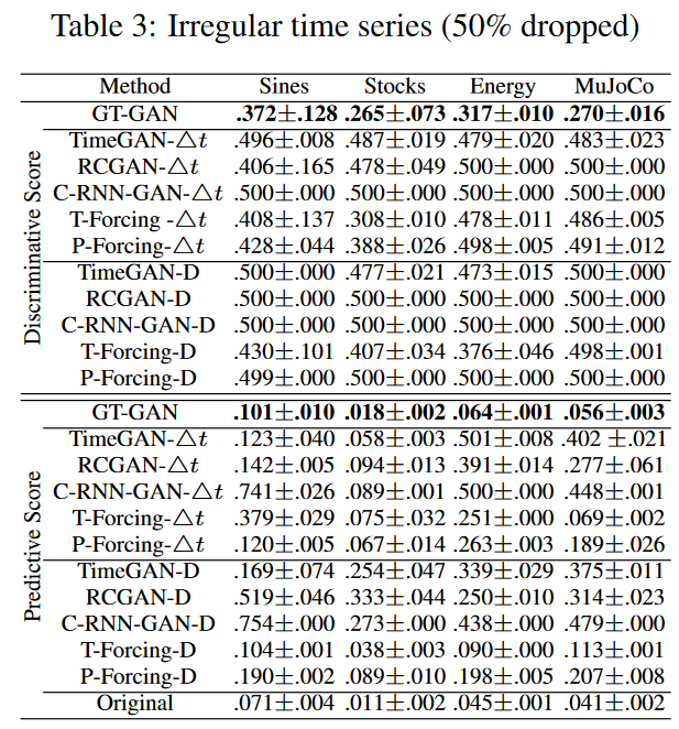
In Table 3 (50% drop), many baselines did not show reasonable composite quality, e.g., TimeGAND, TimeGAN-4t, RCGAN-D, C-RNN-GAN-D, and C-RNN-GAN-4t had a discrimination score of 0.5. Surprisingly, T-Forcing-D, T-Forcing-4t, P-Forcing-D, and P-Forcing-4t perform well in this case. However, the model of this method performs best across all data sets, with the baseline modified with GRU-4t performing slightly better in this case than the baseline modified with GRU-Decay.
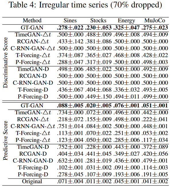
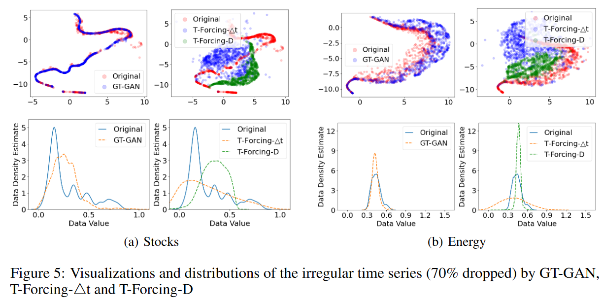
Finally, Table 4 (70% dropped) is the result of the most challenging experiment in this paper. All baselines do not perform well due to high drop rates, although T-ForcingD, T-Forcing-4t, P-Forcing-D, and P-Forcing-4t show reasonable performance with drop rates not exceeding 50%. This indicates that they are vulnerable to highly irregular time series data. Other GAN-based baselines are similarly vulnerable. Our method significantly outperforms all existing methods, e.g., Sines' identification score of 0.278 for GT-GAN, 0.436 for T-Forcing-D, and 0.288 for P-Forcing4t; MuJoCo's prediction score of 0.051 for GT-GAN, 0. 114 and 0.053 for T-Forcing4t. Fig. 5 shows a visual comparison of our method and the best-performing baseline.
Isolation and Sensitivity Analysis
GT-GAN features MLE learning using negative log density in equation (8) and a pre-training step for the encoder and decoder. Table 5 shows the modified results of various GT-GANs with some learning mechanisms removed. The models with negative log density learning perform better than those without. In other words, MLE learning makes the synthetic data closer to the real data. Without pre-trained autoencoders, the prediction score is better than GT-GAN. However, the discrimination score is the worst.
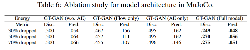
In Table 6, the architecture of the model for this method is modified.
i) In the first carve-out model, the autoencoder is removed and adversarial learning is performed using only the generators and discriminators (called GT-GAN (w.o. AE)).
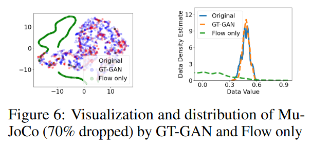
ii) The second carving model (GT-GAN (Flow only)) has only a CTFP-based generator and is trained by the maximum likelihood method. This model is equivalent to the original CTFP model [Deng et al., 2020].
iii) The third carving model has only an autoencoder and is denoted as "GT-GAN (AE only)". However, it is converted to a VAE (variational autoencoder) model: in the full GT-GAN model, the encoder generates the hidden vector {(ti,hreal i ) }N i=0, but in this carve-out model, it is changed to {(ti, N ( hreal i, 1)) }N i=0 and where N ( hreal i, 1) is taken to mean the unit Gaussian centered at hreal i. The decoder is the same as in the full model. Variational learning is used for this model.
Among the separation models, the GT-GAN (Flow only) outperforms the discriminator scores in most cases. However, the full model of this method is the best in all cases. The study in this paper shows that the GT-GAN truncation model does not perform as well as its full model when any part is missing, as shown in Table 6.
Hyperparameters that significantly affect model performance are the absolute tolerance of the generator (atol), the relative tolerance (rtol), and the period of MLE training (PMLE). atol and rtol determine the error control performed by the ODE solver in the CTFP. The results show that there are appropriate error tolerances (atol and rtol) depending on the data input size. For example, we find that datasets with small input sizes (e.g., Sines, Stocks) obtain good discrimination scores at (1e-2, 1e-3) and datasets with large input sizes (e.g., Energy, MuJoCo) at (1e-3, 1e-2).
Related Research
GAN is one of the most representative generation techniques. Since its first introduction in a seminal research paper, GANs have been employed in a variety of major fields. In recent years, the synthesis of GANs for time-series data has been the focus of much attention. Therefore, several GANs have been proposed for the synthesis of time series data: the C-RNN-GAN [Mogren, 2016] has the usual GAN framework applicable to sequential data by using LSTMs as generators and discriminators; the Recurrent Conditional GAN (RCGAN [Esteban et al., 2017]) takes a similar approach, except that its generator and discriminator take conditional inputs for better synthesis; WaveNet [van den Oord et al., 2016] also uses extended casual convolution with to generate time series data from conditional probabilities of historical data.
WaveGAN [Donahue et al., 2019] is a similar approach to DCGAN [Radford et al., 2016] and its generator is based on WaveNet; although it is not a GAN model, it can be modified to generate time series data from teacher-forcing (T-Forcing [Graves, 2014]) and professor-forcing (P-Forcing [Lamb et al., 2016]) models can be modified to generate time series data from noise vectors using their predictive properties; TimeGAN [Yoon et al., 2019] is a further another model for time series synthesis. This model is primarily aimed at synthesizing spurious normal time series samples. They proposed a framework in which GAN is adversarial and supervised learning to predict xi+1 from xi, where xi andxi+1 refer to two multivariate time series values at time ti andti+1, respectively.
summary
Time series synthesis is an important research topic in deep learning and has been studied separately for regular and irregular time series synthesis. However, no existing generative model exists yet that can handle both regular and irregular time series without model modification. The proposed method, GT-GAN, is based on various advanced deep learning techniques ranging from GAN to NODE and NCDE and is capable of handling all possible types of time series without model architecture or parameter changes. Experiments incorporating various synthetic and real-world datasets have proven the effectiveness of the proposed method. In a study of truncation, only the complete method without missing parts showed reasonable synthesis ability.
(Article author) The stability of the entire complex model when training is not detailed, but the neural control differential equation and ordinary differential equation portions are assumed to be good settings and stable.


Categories related to this article