Graphs Are So Awesome! Review Of Integration With Deep Learning
3 main points
✔️ Applications are rapidly advancing due to the expressive power of GNN.
✔️ A review of the deployment of traditional deep learning methods to the flexible and complex structure of GNNs.
✔️ On the other hand, there are ongoing challenges common to deep learning and inherent to graphs
Graph Neural Networks: A Review of Methods and Applications
written by Jie Zhou, Ganqu Cui, Shengding Hu, Zhengyan Zhang, Cheng Yang, Zhiyuan Liu, Lifeng Wang, Changcheng Li, Maosong Sun
(Submitted on 20 Dec 2018 (v1), last revised 9 Apr 2021 (this version, v5))
Comments: Published on AI Open 2021
Subjects: Machine Learning (cs.LG); Artificial Intelligence (cs.AI); Machine Learning (stat.ML)
code:

first of all
Many of you may not be familiar with "graphs" yet. Recently, I have been reading a lot of papers on multivariate time series, and I have noticed that graphs play a major role.
Graph theory itself was first introduced by Euler for one-stroke problems such as Königsberg's Seven Bridges and has been widely applied to route maps, PERT diagrams for project progress plans, molecular structure analysis, linguistics, four-color problems, and web traffic analysis. In the analysis of fake news introduced in the Nikkei Shimbun, the graph structure was focused on. On the right is fake news.
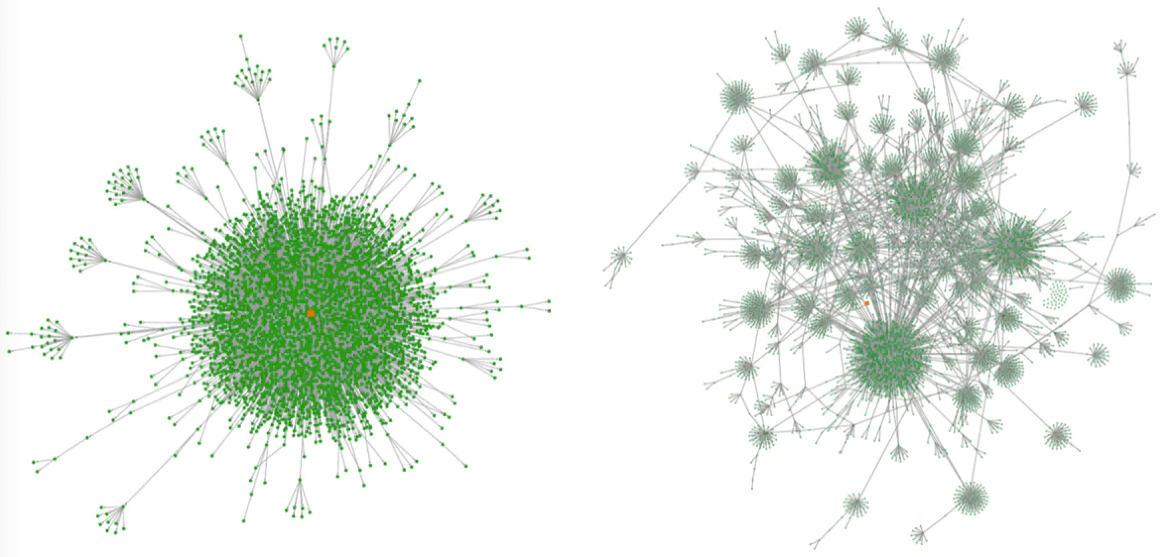
Nihon Keizai Shimbun article: Fakes revealed: A hive of misinformation undermining social networking sites
Looking at the definition, a graph is a data structure represented by objects (nodes) and the relationships (edges) between them.
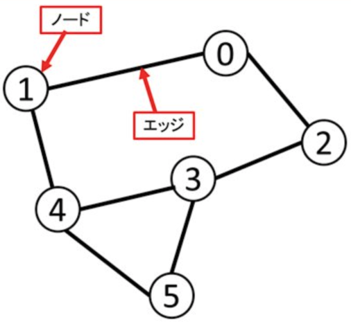
Note: Visualizing Connections: An Introduction to Graph Theory
In the past, deep learning has mainly dealt with collections of individual data (vectors), data arranged in a grid (images), and sequential data (text, voice), but it lacks expressive power when targeting various phenomena and data in the world. I suppose that it was natural to incorporate and develop graph theory.
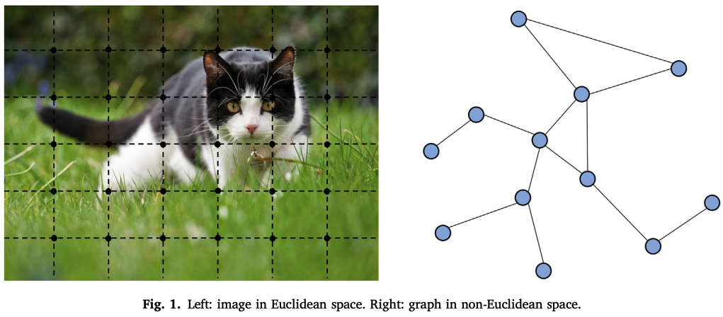
For example, many graph-based GNN (Graph Neural Network) models are emerging in multivariate time series. In addition, machine learning in the form of graphs is receiving more and more attention in many other fields, such as social sciences, natural sciences, and knowledge graphs. In Fig. 1, we can see that a CNN can process local data separated by a grid, and after several layers of CNNs, we can get a complete picture of the "cat". On the other hand, in a graph, Euclidean distance is irrelevant, and the data points related to the "cat" can be combined and treated as a data set.
Another feature is representation learning. Low-dimensional vectors can represent nodes, edges, and subgraphs. In the domain of graph analysis, traditional methods of machine learning rely on the manual setting of feature values, whereas graph embedding methods can be trained; DeepWalk, Skip-gram model, node2vec, LINE, TADW are some examples. However, they also have drawbacks: they are inefficient due to the lack of parameter sharing between nodes, and direct embedding lacks generalization capabilities. From this point of view, various GNN forms have been proposed, and the history of their innovations is overviewed in this paper. Please try to feel the recent trend.
Before we get into the main text, let's talk about the matrix representation for handling graphs mathematically. The adjacency matrix A expresses whether there is a connection relationship between nodes. The degree matrix D represents how many edges are connected to each node. The Laplacian matrix is a representation of these together, L=D-A. The normalized Laplacian matrix is actually used to normalize the Laplacian matrix. Although it looks complicated, it is surprisingly simple when you look at the example implementation.

normalized Laplacian matrix

Wikipedia: Laplacian matrix
This paper is organized as follows.
- A general GNN design pipeline (procedure)
- Materialization of computational modules
- A variant on graph types and scales
- A variant on learning settings
- Design example
- Theoretical and empirical analysis
- Main Applications
- Four unresolved issues
Many of the forms will be presented in 3. The original paper is 25 pages long, so it is a bit lengthy, but please bear with us.
GNN General Design Pipeline
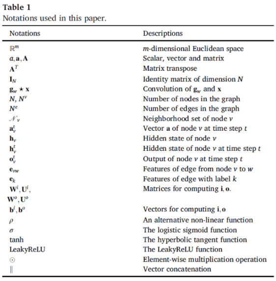
First, let's look at it from the designer's point of view. We denote a graph as G=(V, E). Here, the size N of V is the number of nodes, the size $N^e$ of E is the number of edges, and A is the adjacency matrix. For learning the representation of the graph, we use the hidden state of node v and the output vectors $h_v, o_v$. Table 1 shows the notation used in this paper.
Graph Structure
The structure of the graph is found in the application. There are usually two scenarios: structural and non-structural. In the former, the structure of the application is explicitly represented, e.g. molecular structures, physical systems. In the latter, e.g. for words, images, the model is first created in full coupling and then optimized.
Graph types and scales
The next step is to determine the type of the graph and the scale. A graph with a complex type can have more information due to its nodes and connection relationships.
Graphs with and without direction
In a directed graph, every edge has a direction. An edge in an undirected graph can also be considered a bidirectional edge.
Homogeneous and heterogeneous graphs
In a homogeneous graph, all nodes and edges are of the same type.
Static and dynamic graphs
A graph is considered dynamic if the input feature values and the graph connectivity change over time.
There is no clear classification criterion for scale. Here, we consider the scale at which the adjacency matrix, or graph Laplacian, cannot be stored in the processing device to be large, and some sampling technique is required.
loss function
The loss function is determined by the task type and learning settings.
Node level
It focuses on nodes. It includes node classification, node regression, and node clustering.
Edge level
There are two types of edge prediction: edge classification, which classifies edge types, and link prediction, which predicts the existence of an edge between two given nodes.
Graph level
These are graph classification, regression, and clustering. All of these require a model to learn the graph representation.
In terms of supervised data, all of the usual types of machine learning exist. They are "supervised", "semi-supervised" and "unsupervised". In "semi-supervised" learning, We have a small number of labeled nodes and a large number of unlabeled nodes for training. In the testing phase, the Transductive setting requires a model that predicts labels given unlabeled nodes. On the other hand, in the inductive setting, a new unlabeled node is prepared and inferred. Recently, a mixed Transductive-inductive scheme has been introduced.
compute module
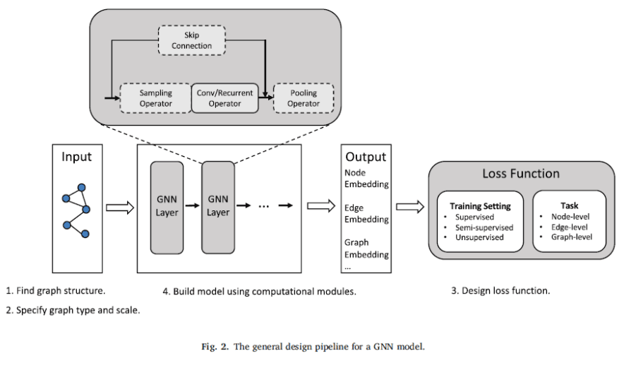
The commonly used computational modules are the propagation module, the sampling module, and the pooling module. By combining these modules, a typical GNN is designed as the middle part of Fig. 2. To increase the expressive power, a multilayer structure is usually adopted. Some models do not fit this general form.
Materialization of computational modules
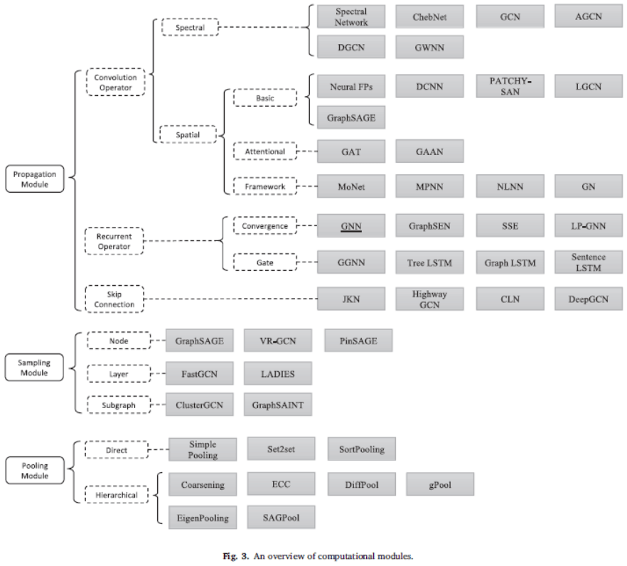
According to the classification in Fig. 3, we introduce various GNNs in the form of calculation modules.
Propagation Module - Convolution
There are two ways to generalize convolutional operations and apply them to graphs: spectral approaches and spatial approaches.
・Spectral
to the spectral space. The Fourier transform and the inverse Fourier transform are denoted as
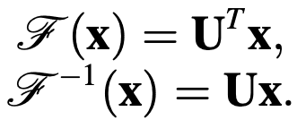
$U$ is the eigenvector matrix of the normalized graph Laplacian.
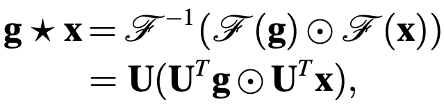
The convolution operator is defined as follows
Using the diagonal matrix $G_W$, the basic function of the spectral method is represented as follows. The procedure is to Fourier transform, apply filter $G_M$, and inverse Fourier transform.
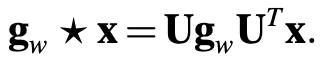
Typical spectral methods using various $G_W$ are as follows.
Spectral Network uses a diagonal matrix $g_w = diag(w)$ as a filter. It is considered to be computationally inefficient.
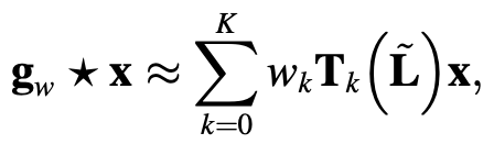
In contrast, ChebNet proposes the $g_m$ polynomial Chebyshev polynomial in powers of cos(x), censored at degree k.
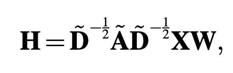
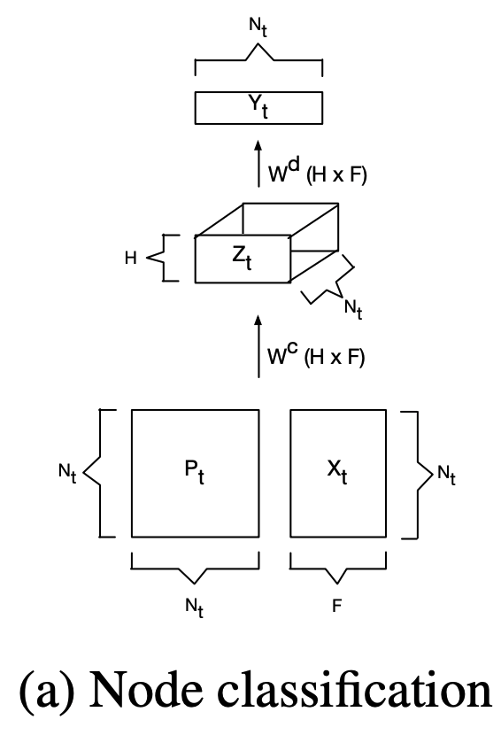
GCN (Graph Convolution Networks ) further censors the above equation up to k=1 to reduce the overfitting problem. It can be further simplified to This is the beginning of the spatial approach described in the next section, where H is the convolution matrix, X is the input matrix, and W is a parameter.
AGCN (Adaptive Graph Convolution Network) is a method that attempts to learn implicit relations, adding the residual graph Laplacian to the original Laplacian. It is efficient for molecules and chemical compounds.
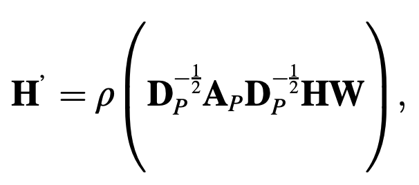
The Dual Graph Convolution Network ( DGCN ) captures both local and global relationships. (PPMI) matrix. $A_p$ is the PPMI matrix and $D_p$ is the corresponding order matrix.
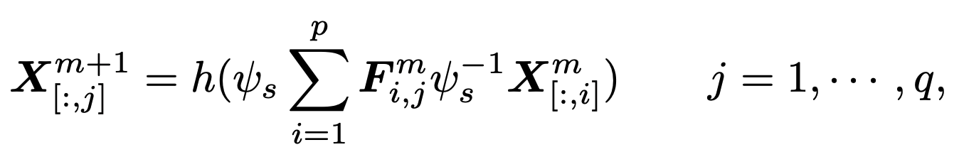
GWNN (Graph wavelet neural network) uses the graph wavelet transform $\psi _s$ instead of the graph Fourier transform. The advantages are that the wavelets can be obtained without matrix factorization, the graph wavelets are sparse and localized, and the results are highly explanatory.
Spectral approach methods have clear theoretical underpinnings, but the problem is that the filters depend on the graph structure and cannot be applied to other graph structures.
Basic spatial approach
The spatial approach defines convolution directly based on the topology of the graph, in this case, the connection form. The main challenge is to define convolution operators for neighbors of different sizes and to preserve local invariants.
Neural FPs use different weight matrices for nodes with different degrees. It has the disadvantage that large graphs are difficult to handle. We evaluate the performance against chemical compounds.
DCNN (Diffusion convolution neural network) defines the adjacency of nodes by a transition matrix (or probability matrix ) It is used to classify nodes, graphs, and edges. It is used for the classification of nodes, graphs, and edges.
PACHY-SAN extracts and normalizes the adjacencies of exactly k nodes for each node. It acts as a receptive field for normal convolution.
LGCN (Learnable graph convolutional network) extracts top-k feature values by max-pooling of adjacency matrices and applies 1D CNN to compute the hidden layer by hidden representation.
GraphSAGE is a general inductive framework, collecting feature values from local neighbors of nodes (aggregators). three types of aggregators have been proposed. Three types of aggregators have been proposed: average, LSTM, and pooling.
Attention Base
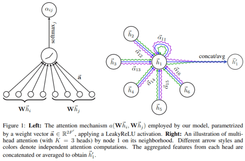
Graph attention network ( GAT ) has also been applied to multivariate time series (MTAD-GAT ). It incorporates attention between neighboring nodes and also self-attention. Multi-headed attention has also been used.
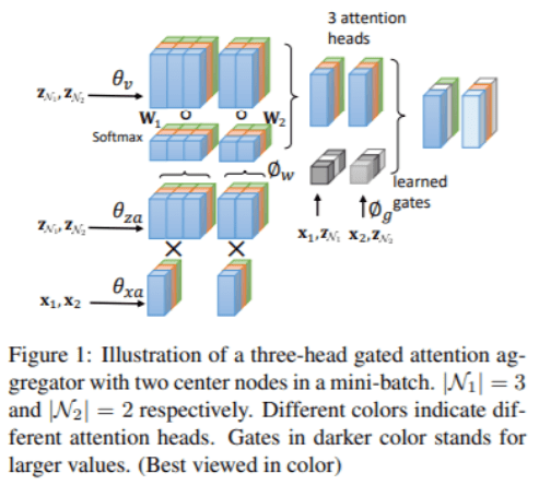
GaAN (Gated attention network) similarly uses multi-headed attention; unlike GAT, the importance of each attention head can be changed.
The general framework of the spatial approach
The proposal is to integrate different models into a single framework.
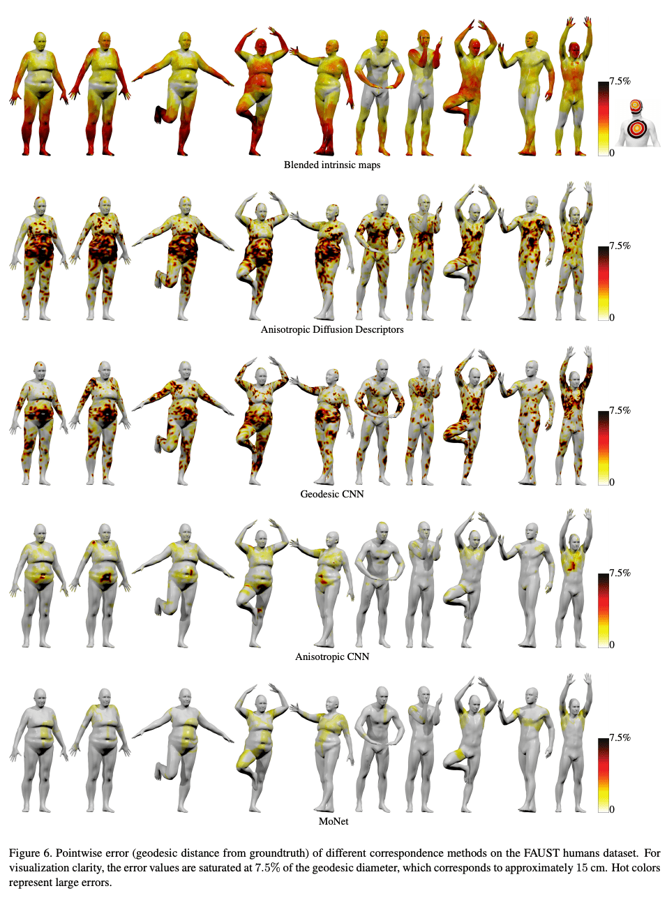
MoNet (Mixture model network) provides a framework for designing convolutional deep architectures in non-Euclidean domains such as manifolds and graphs. Operators are applied locally, like patches. What is novel about this approach is that it chooses different operators depending on the characteristics of each local. Examples that can be formulated as entities of this framework include GCNN (Geodesic GNN) and AGNN (Anisotropic GNN) for manifolds, and GGN and DGNN for graphs. The following figure shows the comparison of FAUST human dataset. The colored area is the point where the error occurs, and the bottom MoNet shows the best result.
Message passing neural network (MPNN ) extracts the properties of several classical methods. The method has been developed for quantum chemistry and consists of two phases, the first is message transfer and the second is readout. In the message transfer, messages are collected from neighboring nodes and the hidden variables are updated through an update function. In the readout phase, the hidden variable is output using the read function. By changing the settings of each function, different models can be materialized.
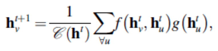
NLNN (Non-local neural network) generalizes and extends the classical non-local mean. Non-local averages compute weighted feature values from all Spatio-temporal points and use them as hidden variables. It can be regarded as a unified form of self-attention. The definition of the operator is as follows, and it can take various forms depending on the choice of f and g.
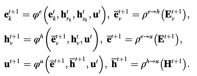
GN (Graph network) learns node level, edge level, and graph level. It can generalize many transformations. The core computational unit is called GN-block and consists of three update functions $\varphi$ and three aggregate functions $\rho$.
Propagation Module - Recursion
Whereas the convolutional layers up to this point have used different weights, the recursion layers share the same weights.
Convergence-based method
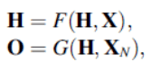
GNN (Graph neural network) initially referred to this technique. Later, it came to refer to a broader range of graph neural networks. To avoid confusion, we distinguish between these methods by underlining them in this paper. For a state H, an output O, a feature value X, and a node feature value $X_N$, the matrix notation for a GNN is.
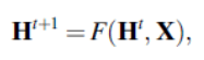
The asymptotic expression is as follows
The limitation of GNN is that F must be a contraction map, which constrains the performance of the model. Also, focusing on the node representation, the use of fixed points is not suitable due to its low information content.
GraphSEN (Graph Echo State Network) is a generalization of the echo state network, which is more efficient than GNN because the convergence is guaranteed by the reservoir layer property of ESN.
Stochastic Steady-state Embedding ( SSE ), which also tries to improve the efficiency of GNNs, proposes a two-step learning process. In the update step, the incorporation of each node is updated by a parameterized operator, and in the mapping step, it is mapped to the steady-state space according to the constraints.
LP-GNN (Lagrangian Propagation GNN) formulates the learning task as a constrained optimization problem in a Lagrangian framework. This avoids recalculating for fixed points.
gate-based method
As in general deep learning, gating mechanisms such as LSTM and GRU are applied to graphs. The computations of each method are summarized in Table 2.
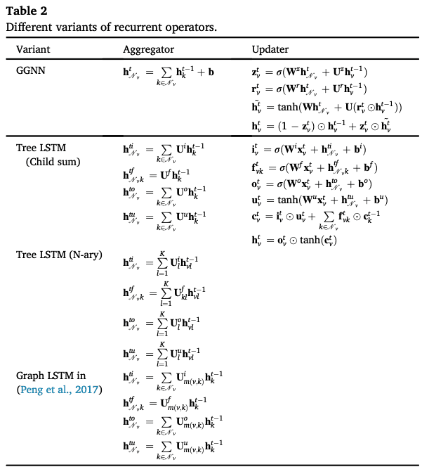
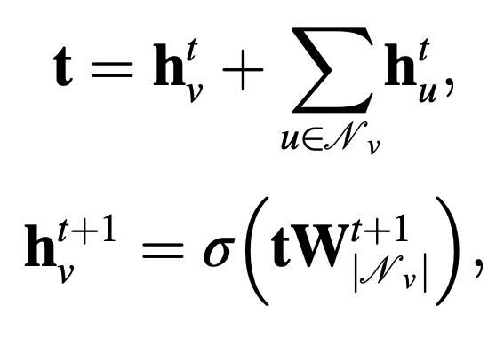
GGNN (Gated graph neural network) tries to release the constraint of GNN, using GRU, gradient calculation by BPTT. The hidden state $h_N_\nu$ of each node collects information about its neighbors.
Tree LSTM has two extended forms, Child-Sum Tree-LSTM and N-ary Tree-LSTM, which have a forgetting gate for each child of the Tree structure.
Graph LSTM is an example of N-ary Tree-LSTM applied to a graph.
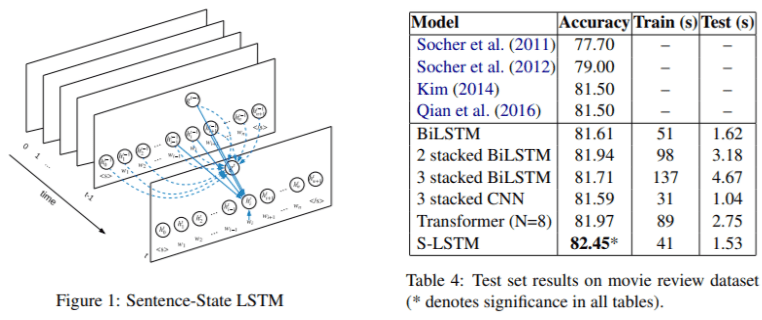
S-LSTM (Sentence LSTM) converts sentences into graphs and learns representations using Graph LSTM.
Propagation Module - Skip Connections
For graph neural networks, too, the aim is to increase the expressive power by deepening the layers, but this does not necessarily improve the performance because of the problems of increased noise and excessive smoothing. Therefore, skip connections are performed as in general deep learning.
Highway GCN uses a Highway Gate for each layer.
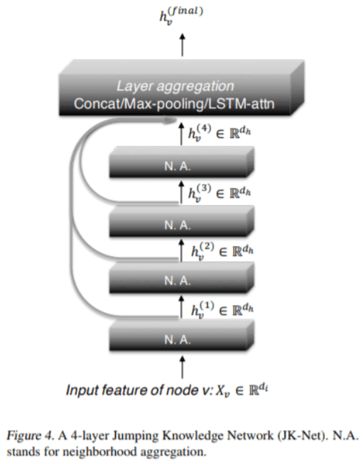
The Jump knowledge network ( JKN ) adaptively selects the Jumps that connect to each node in all intermediate to final layers.
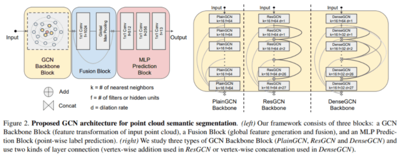
DeepGCN borrows ideas from ResNet and DenseNet to solve the problems of gradient vanishing and over-smoothing.
Sampling Modules
At each layer, aggregating messages from neighboring nodes causes the problem of "neighbor explosion", where the number of nodes involved increases rapidly as the layers overlap. To mitigate this problem, sampling is used.
nodal sampling
GraphSAGE samples only a small number of neighbors.
VR-GCN is a control variable-based stochastic approximation method. It restricts the receptive field to one skipping (1-hop) neighbor.
PinSAGE proposes importance-based sampling. A random walk restricts the neighboring nodes to the top T of the average number of visits.
Stratum sampling
FastGCN samples the receptive fields of each stratum directly.
LADIES ( LAyer-Dependent Importance Sampling ) samples from adjacent joins of nodes.
Subgraph sampling
ClusterGCN clusters the graph and samples the subgraphs.
GraphSAINT samples nodes or edges directly to form subgraphs.
pooling module
As in the Computer vision method, pooling is applied to obtain more general feature values.
Direct pooling
Simple Node Pooling performs the maximum, average, sum, and attention operations on the feature values of each node.
Set2set is used in the readout function of MPNN, which handles unordered sets and generates order invariants using LSTM-based methods.
SortPooling sorts node embeddings according to the structural role of the node and sends them to the GNN.
Hierarchical pooling
Graph Coarsening is an early method that uses node clustering as pooling.
Edge-Conditioned Convolution ( ECC ) performs recursive downsampling. It divides the graph into two elements according to the polarity of the maximum eigenvalue of the Laplacian.
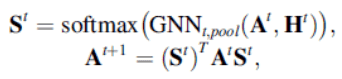
DiffPool uses a learnable hierarchical clustering module to coarsen the adjacency matrix using the following assignment matrix $S^t$.
gPool uses the mapping vector to learn the mapping score of each node and selects nodes from the top k scores.
EigenPooling combines node feature values and local structures. It extracts subgraphs by local Fourier transform.
SAGPool (Self Attention Graph Pooling) also uses feature values and topology together to learn a graph representation. It uses a self-attention-based method.
Transformations on graph types and scales
According to Fig.4, we introduce various GNNs by graph type and scale.
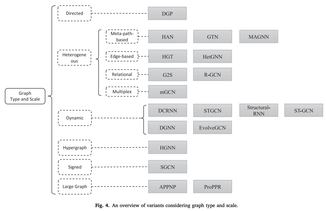
directed graph
It is more informative than an undirected graph. For example, in a knowledge graph, the head entity is the parent class of the tail entity. The direction of the edge represents the parent-child relationship. It is possible to model forward and reverse edges separately. (DGP)
heterogeneous graph
Meta path base
A meta-path is a routing scheme that determines the type of nodes at each location along the path. During training, it is materialized as an ordering of nodes. By connecting the nodes at both ends of the meta-path, we can figure out the similarity between two nodes that were not directly connected. One heterogeneous graph may be reduced to several homogeneous graphs.
The Heterogeneous graph Attention Network ( HAN ) applies attention to meta-path-based neighbors and semantic attention to output embedding under all meta-path schemes to produce a final representation of the nodes.
MAGNN (Metapath Aggregated Graph Neural Network) takes into account the intermediate nodes of a meta-path. After aggregating the information along the meta-path, it takes the attention along the related meta-path.
GTN (Graph Transformer Networks) proposes a method of graph transformation. It defines connections between unconnected nodes while learning to represent them.
edge-based
HGT (Heterogeneous Graph Transformer) defines a meta-relationship as a type of two adjacent nodes and their connections. Different meta-relationships are assigned different attention weight matrices.
HetGNN ( Heterogeneous Graph Neural Network ) deals with different types of neighboring nodes with different sampling, feature value encoding, and aggregation steps.
Relationship graph
G2S (Graph-to-Sequence) transforms the original graph into a graph divided into two parts. Then, GGNN and RNN are applied to transform the graph into a sentence.
R-GCN (Relational Graph Convolutional Networks ) assigns different weight matrices to the propagation of different types of edges. We introduce two constraints to limit the number of parameters. In the basic decomposition, $W_r=\sum_{b=1}^B a_{rb} V_b$. In the block diagonal decomposition, we define $W_r$ to be the direct sum over the low-order matrix set.
-multiplexed graph
mGCN (Multi-dimensional Graph Convolutional Networks) introduces a general representation and a dimension-specific representation in each layer of GNN. Dimension-specific representations are mapped from the general representation by different mapping matrices. They are then aggregated to form the general representation of the next layer.
dynamic graph
DCRNN (Diffusion Convolutional Recurrent Neural Network), STGCN (Spatio-Temporal Graph Convolutional Networks) first collects the spatial information of GNN, and the output is the sequential data.
Structural-RNN, ST-GCN (Spatio-Temporal Graph Convolution), collect spatial and temporal messages simultaneously and extends the static graph structure to temporal connections.
DGNN (Dynamic Graph Convolutional Networks) gives the built-in output of each node of GCN to LSTM.
EvolveGCN feeds GCN weights to the RNN to capture genuine graph interactions.
Other graph types
Hypergraph
In Hypergraph Neural Networks ( HGNN ), edges are combined with multiple nodes with their own weights.
Polarity graph
SGCN (Signed Graph Convolutional Network) uses balance theory to understand the interrelationship between positive and negative edges. Intuitively, a friend of a friend is a friend of a friend, and an enemy of an enemy is a friend of an enemy.
large graph
Sampling is one method for large graphs, but other methods include packing multiple GCN layers into a single propagation layer in PageRank and precomputing convolutional filters of different sizes.
Transformations for different learning settings
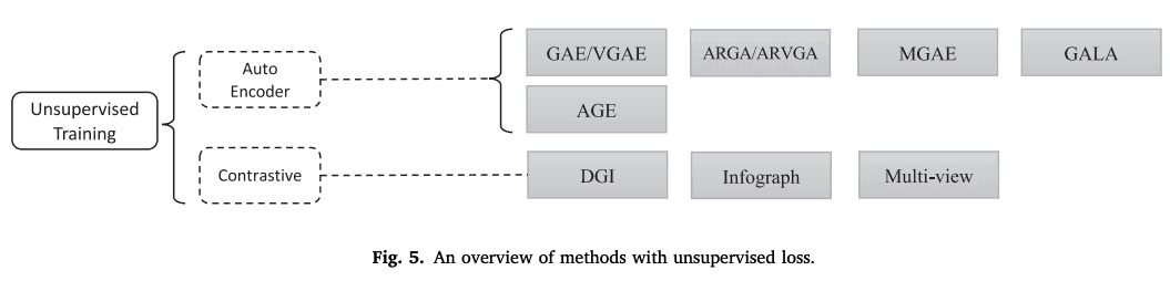
Graph Auto Encoder
GAE/VGAE first encoded the nodes using GCN, recovered the neighbors with a simple encoder, and calculated the difference from the original neighbors as the error.
ARGA (Adversarially Regularized Graph Auto-Encoder)/ARVGA is a GCN-based graph auto-encoder with GAN applied.
MGAE (marginalized graph auto-encoder) is a robust node representation using a marginalized denoising auto-encoder.
GALA decodes the hidden states using Laplacian sharpening, the inverse of Laplacian smoothing. This method reduces the problem of over-smoothing in GNN learning.
AGE performs adaptive learning by measuring the similarity of nodes per pair, as the restoration loss is independent of the downstream task.
Contrastive Learning
Contrastive learning is another stream of unsupervised graph representation learning.
DGI (Deep Graph Infomax) maximizes the mutual information between node representation and graph representation.
infograph performs graph representation learning by maximizing the mutual information between graph-level representations and substructure representations at different scales, such as nodes, edges, and triangles.
Multi-view contrasts and learns to represent first-order adjacency matrices and graph diffusions.
GNN design example
Taking GPT-GNN as an example, the design process of GNN is as follows.
1. Find the graph structure
We focus on the application of academic knowledge graphs and recommendation systems. In a recommendation system, users, items, and reviews are defined as nodes and their relationships as edges.
2. Decide the graph type and scale
This task focuses on heterogeneous graphs. There are millions of nodes and we will be dealing with large heterogeneous graphs.
3. Designing the loss function
Since all downstream tasks are node-level, we need to pre-train the node representation. In pre-training, we design self-supervised learning with no label data. In fine-tuning, we train on the data of each task.
4. Build the model using the calculation module
The propagation module is the convolutional operator HGT, the sampling module is the specially designed HGTsampling, and the pooling module is not used since it learns the node representation.
GNN Analysis
theoretical viewpoint
Graph signal processing
From a signal processing perspective, the Laplacian has the effect of a low-pass filter. It reflects the similarity hypothesis, that nearby node are assumed to be similar.
generalization (psychology, linguistics, etc.)
For generalization performance, the VC dimension has been proved for some GNNs; a tighter generalization limit has been given by Garg et al. based on the Rademacher limit for neural networks; the stability of GNNs is said to depend on the maximum eigenvalue. Attention helps the generalization of GNNs for larger and noisier graphs.
Expressiveness
Xu et al. show that GCN, GraphSAGE, is less expressive than the Weisfeiler-Leman test, an algorithm for testing graph homomorphic mappings, and Barcelo et al. show that GNNs are hardly compatible with FOC2, a fragment of first-order predicate logic. Regarding the topological structure of the learning graph, they state that locally dependent GNN forms are unable to learn global graph properties.
Invariance
Due to the unordered nature of the nodes, the GNN output embedding is equivalent to the permutation invariants or the input feature values.
・Convertibility
Since parameterization is not tied to graphs, it is suggested to convert between graphs based on performance guarantees.
Label efficiency
The (semi-)supervised learning of GNNs requires a very large amount of labeled data to satisfy the performance. Methods to increase the efficiency of labeling have been studied, and the efficiency can be dramatically improved by selecting high order nodes, uncertain nodes, and other information-rich nodes.
empirical viewpoint
Evaluation
Note that the ranking may change or become an inappropriate comparison depending on how the data is divided and the condition setting.
Benchmark
For graph learning, widely accepted benchmarks are hard to come by. Most node classification datasets contain only 3,000 to 20,000 nodes, which is smaller than real-world graphs. Experimental procedures are also not standardized. However, reliable benchmarks have recently become available.
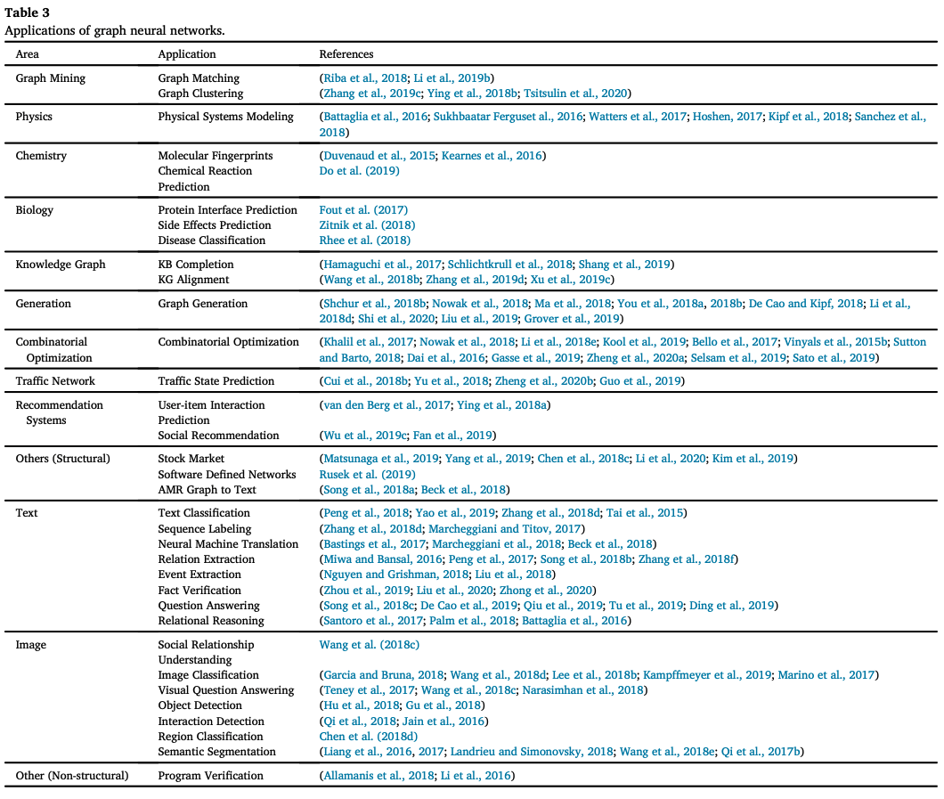
application
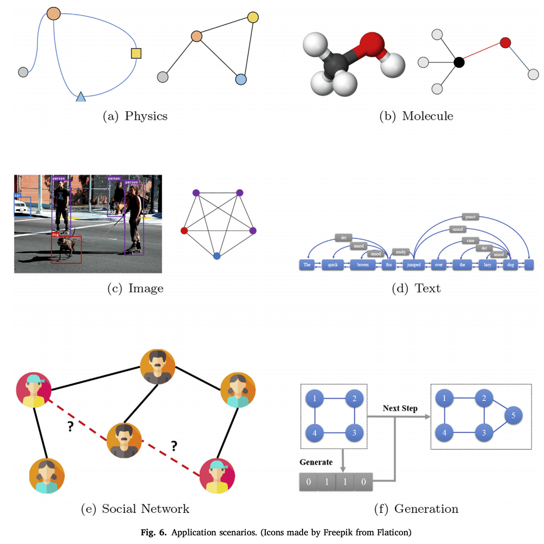
Structural Scenarios
Graph Mining
Graph mining includes subgraph mining, graph matching, graph classification, and graph clustering. For graph matching, the high level of computational complexity has been a challenge, but with the advent of GNNs, it is now possible to use neural networks to understand graph structure. A recent example of graph clustering studies the characteristics of good clustering, and optimization of spectral modularity has been proposed, which is a good metric.
・Physics
Simulating a physical system requires a model that learns the laws of the system. The system can be simplified as a graph by modeling the objects as nodes and the interrelationships between each pair as edges. Examples include particle models, robots; NRIs take object trajectories as input and infer explicit interrelationship graphs; Sanchez et al. proposed a graph network that encodes the body and joints of a robot. It is coupled with reinforcement learning.
Chemistry, Biology
In molecular fingerprinting, Neural PPs and Kearnes et al. compute substructure feature value vectors by GCN and explicitly model atom pairs, respectively, to highlight atomic interactions.
In chemical reaction prediction, the Graph Transformation Policy Network encodes the input molecules and the node-pair prediction network generates the intermediate graph.
In protein boundary prediction, the representations of ligand and receptor proteins are learned by GCN and classified by pairs, or local and global feature values are predicted by a multi-resolution approach.
In biomedical engineering, the Protein-Protein Interaction Network uses graph convolution to classify breast cancer, and Zitnik et al. create a GCN-based model for predicting side effects of multidrug combinations.
Knowledge Graph
The Knowledge Graph (KG) is a collection of real-world entities, representing the relationships between entity pairs. The Structure-Aware Convolution Network combines a GCN encoder with a GNN decoder to improve knowledge representation. Hamaguchi et al. apply GNNs to the problem of out-of-knowledge-base (OOKB) in the task of completing entities that are not explicit in the training data (KBC).
On the other hand, Wang et al. apply GGNs to align knowledge graphs across different languages; OAG uses graph attention networks for this task; Xu et al. replace this problem with a graph matching problem, and Xu et al.
Generative model
Generative models are of growing interest in social interaction modeling, new chemical discovery, knowledge graph construction, etc. NetGAN generates graphs by random walks; GraphRNN generates adjacency matrices by the step-by-step generation of adjacency vectors for each node. GraphAF formulates graph generation as a sequential decision process.
The GCPN (Graph Convolutional Policy Network) uses reinforcement learning.
・Combinatorial optimization
Combinatorial optimization is a well-known problem in graph theory, such as the traveling salesman problem (TSP) and minimum-wide trees. Gasse et al. represented the state of the combinatorial problem as a bipartite graph and used GCN for encoding; Sato et al. performed a theoretical analysis and established the coupling between GNNs and distributed local algorithms. They also showed how far an approximation ratio can be reached by the best optimization solution. Several specialized models for specific problems have also been proposed.
Transportation Network
Prediction is challenging because transportation networks are dynamic and have complex dependencies. Cui et al. combined GNN, LSTM to understand the temporal and spatial dependencies. STGCN uses ST-Conv blocks for spatial-temporal convolution. There is also an attempt to use Attention.
Recommended system
User and goods interactions are modeled using graphs; GC-MC was the first model; PinSage uses a bipartite graph weighted sampling strategy to reduce computational complexity; GraphRec uses SNS information; Wu et al.'s method models similarity and influence effects using two modelings with attention.
Other structural applications
In financial markets, it is used to model the relationship between different stock prices and to predict the future. Software-Defined Networks is used for routing, Abstract Meaning Representation is used for sentence generation.
Unstructured scenario
・Image
In Few(Zero)-shot image classification, the GNN approach is to exploit the richer information using graphs, one using knowledge graphs and the second using similarity between images.
A typical task in image reasoning is Visual Question Answering (VQA); Tenney et al. constructed an image scene graph and a question syntax graph and predicted the answers using GGNN.
In semantic segmentation, Liang et al. modeled long-term dependencies and spatial connections by building graphs in the form of interval-based spar pixel maps using graph LSTM.
plain text
In sentence classification, graphs can figure out the meaning between non-contiguous, distant words.
Sequence labeling gives a categorical label to a sequence of observed variables. If we consider variables in a sentence as nodes and dependencies as edges, we can capture this problem as a hidden state of GNN.
The use of GNNs in machine translation is to add syntactic and semantic information.
About extraction, in a sentence graph, nodes correspond to words, and edges can be fitted with adjacencies, syntactic dependencies, and dialogue relations.
Event Extractor extracts events from a sentence.
Fact-finding extracts the evidence that supports the claim.
Unresolved Issues
Robustness
As a family of neural networks, GNNs are also vulnerable to adversarial attacks. Research on attacks and defenses against graph structures has begun. See our comprehensive review.
interpretability
The black-box nature of GNNs is also strong, and there are only a few explanations of the model on an example bases.
Graph pre-study
Preliminary studies on graphs have just been initiated. Those studies also have different problem settings and perspectives, and still, require extensive research.
Complex graph structures
For real-world applications, graphs are becoming more flexible and complex. Dynamic and heterogeneous graphs have been introduced here, but more powerful models are needed.
summary
Graph-based neural networks are not easy to understand, but they can handle atypical and complex data that cannot be handled by MLP, CNN, etc. Therefore, research and application of graph-based neural networks have been rapidly progressing in recent years. This review paper shows that most of the deep learning, CV, NLP, and other methods have been deployed in graph-based systems.
On the other hand, there are still challenges common to deep learning and specific to graph neural networks that warrant further research. Links to the source code of the main GNN models presented here can be found in the appendix of the paper. Frameworks for graph computation have also been developed and are surprisingly simple to implement.


Categories related to this article