Can We Trust The Output Probability Of A Classifier? "AdaFocal" Loss Function To Improve Calibration Performance
3 main points
✔️ Proposed AdaFocal to adaptively adjust the hyperparameter γ of Focal Loss
✔️ Achieved higher calibration performance than existing methods while maintaining comparable classification performance
✔️ Confirmed effectiveness in out-of-distribution detection tasks
AdaFocal: Calibration-aware Adaptive Focal Loss
written by Arindam Ghosh, Thomas Schaaf, Matthew R. Gormley
(Submitted on 21 Nov 2022 (v1), last revised 16 Jun 2023 (this version, v2))
Comments: Published in NeurIPS 2022.
Subjects: Machine Learning (cs.LG); Computer Vision and Pattern Recognition (cs.CV)
code:
The images used in this article are from the paper, the introductory slides, or were created based on them.
Introduction.
The classification problem of estimating which category data belongs to is one of the typical tasks in which machine learning is utilized. For example, a possible problem is to determine whether something in an image is a dog or a cat. For this problem, the machine learning model calculates the probability that the object is a dog and the probability that it is a cat, and determines that the object with the higher probability is the one in the image. For a variety of classification problems, machine learning models have achieved over 90% classification performance.
But are the probabilities used in the classification correct?
For example, if we collect samples that are judged to be "90% dog," do we really get the result that 10% of them are not dogs? In recent years, research has been conducted on the calibration problem, which is to match the output probability of a classifier with the correct probability. In this paper, we propose Ada Focal, an improved version of Focal Loss, to further improve calibration.
Calibration Evaluation Methods
This section describes the evaluation indicators in the calibration problem.
With a finite data set, it is not possible to determine the exact calibration error (CALIBRATION ERROR). Therefore, an estimate of the calibration error is used for evaluation. There are various estimation methods, but here we explain the Expected Calibration Error (ECE) , which is mainly used in this paper.
![]()
The ECE is obtained by calculating the calibration error for each sample group with close probabilities and summing them, where M is the number of sample groups [1] and N is the number of total (evaluation) data.
Bi represents the data set contained in the i-th sample group; ECEEM divides all sample groups so that the number of samples is the same (EM: Equal Mass), as in the following equation.
![]()
Ai represents the percentage of correct answers in sample group Bi.
![]()
Ci represents the mean probability in sample group Bi.
![]()
Focal Loss
This section describes Focal Loss, which is the basis of the proposed method (AdaFocal).
summary
Focal Loss was initially proposed to improve classifier performance by reducing the training weights for easy samples (easy samples) in Cross Entropy Loss and allowing intensive training of hard samples (hard samples ). Focal Loss can be expressed as follows
![]()
The equation is formed by multiplying the Cross Entropy Loss, -logp, by (1-p) γ. The closer p is to 1 (easy sample), the smaller the value of (1-p)γ becomes, and thus the relative weight of hard sample can be increased. The closer p is to 1 (easy sample), the smaller the value of (1-p) γ becomes, which means that the weight of the hard sample can be relatively larger. γ is a hyperparameter that adjusts the difference between the weights of the easy sample and the hard sample. It is the same as Cross Entropy Loss.
Calibration characteristics
Subsequently, it was also shown that Focal Loss has the effect of improving calibration. The reason for this can be explained using the following relationship
![]()
From the above equation, we can see that decreasing Focal Loss reduces KL Divergence and increases the entropy of the prediction vector p. This is believed to improve calibration by preventing the model from overconfidently making incorrect predictions.
issue
The challenge with Focal Loss is how to determine the hyperparameter γ.
The figure below compares the accuracy of calibration when ResNet50 is trained on CIFER-10 with Cross Entropy Loss (CE: γ=0), Focal Loss γ=3,4, 5 (FL-3/4/5), and Sample-Dependent Focal Loss (FLSD-53 ) [2], comparing the accuracy of the CALIBRATION when trained with (a) shows the overall evaluation by ECEEM, one of the above mentioned calibration metrics, and (b) shows the change in calibration error per epoch for the sample groups with low (Bin-0), medium (Bin-7), and high (Bin-14) prediction probabilities, respectively. The sample group is shown in (a) and (b).
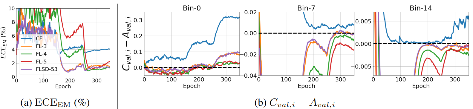
Comparing among (CE, FL-3/4/5) with fixed γ, the graph in (a) shows that overall the best calibration is when γ=4. However, (b) shows that γ=4 is not the best depending on the magnitude of the predicted probability (Bin-7). In other words, it is difficult to determine a single appropriate γ in calibration.
FLSD-53, which varies γ according to the magnitude of the prediction probability, also does not give the best results in all cases of Bin-0, 7, and 14.
From these results, it can be said that it is necessary to define γ in a way that is more appropriate for each level of predictive probability.
Proposed Method
AdaFocal uses Focal Loss as well as Inverse Focal Loss to learn. Before moving on to the explanation of AdaFocal, I will explain Inverse Focal Loss.
Inverse Focal Loss
We explained above that Focal Loss has the effect of preventing the model from being overconfident and making incorrect predictions by reducing the weight on the easy sample. On the other hand, what should we do if the model lacks confidence?
In this paper, we propose to use Inverse F ocal Loss to solve the problem of model underconfidence.
![]()
The term (1-p) in Focal Loss is changed to (1+p) in Inverse Focal Loss. This gives a large gradient to the easy sample, contrary to Focal Loss, and allows the model to be trained to be overconfident.
In AdaFocal, training proceeds by guiding the model to output just the right probability, neither overconfident nor underconfident, by appropriately using both Focal Loss and Inverse Focal Loss.
AdaFocal ~How to update gamma
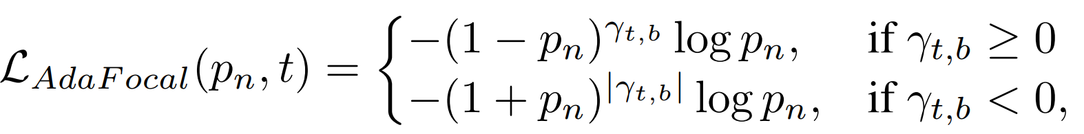
This section describes how AdaFocal adjusts the hyperparameter γ, which was an issue for Focal Loss. the update formula for γ in AdaFocal is as follows
![]()
AdaFocal adjusts γ based on Eval , b = Cval , b - Aval , b, which is the calibration error observed in the validation data.γt is calculated for each sample group that has close output probabilities, and b is the index of the sample group. λ is a hyperparameter that determines how much γ is adjusted per update (epoch). hyperparameter that determines how much γ is adjusted per update (epoch) [3].
The updated formula for γ is designed based on the ideas presented below.
- Cval, b - Aval , b > 0 (Cval , b > Aval ,b ):
Since the output probability of the model tends to exceed the actual percentage of correct answers, the model is trained in such a way that overconfidence in the model is suppressed. Therefore, increase γ so that the weight on the easy sample is reduced. - Cval , b - Aval , b < 0 (Cval , b < Aval ,b):
Since the output probability of the model tends to be lower than the actual percentage of correct answers, the model is trained to be overconfident. Therefore, we decrease γ so that the weight on the easy sample is increased.
We can also expand γt to express![]()
From this equation, we can see that as the number of epochs (t) increases, the value of γt has a tendency to explode. Therefore, upper ( γmax) and lower ( γmin ) limits are set forγt to prevent explosion [4].
AdaFocal ~Switch between Focal Loss and Inverse Focal Loss
As γ is decreased, the weight of the easy sample, which is smaller than the weight of the hard sample, becomes larger and larger (relatively speaking). When γ is further reduced, it is natural that the weight of the easy sample increases relative to the weight of the hard sample. Therefore, we switch to Inverse Focal Loss when γ becomes negative. That is, when γ > 0, the Focal Loss of the parameter γ is used, and when γ < 0, the Inverse Focal Loss of the parameter|γ| is used.
However, in actual training, Focal Loss and Inverse Focal Loss are switched when |γ| falls below the threshold value Sth, even if the positive or negative value of γ does not change [5].
AdaFocal - Summary
The AdaFocal algorithm described so far can be summarized as follows.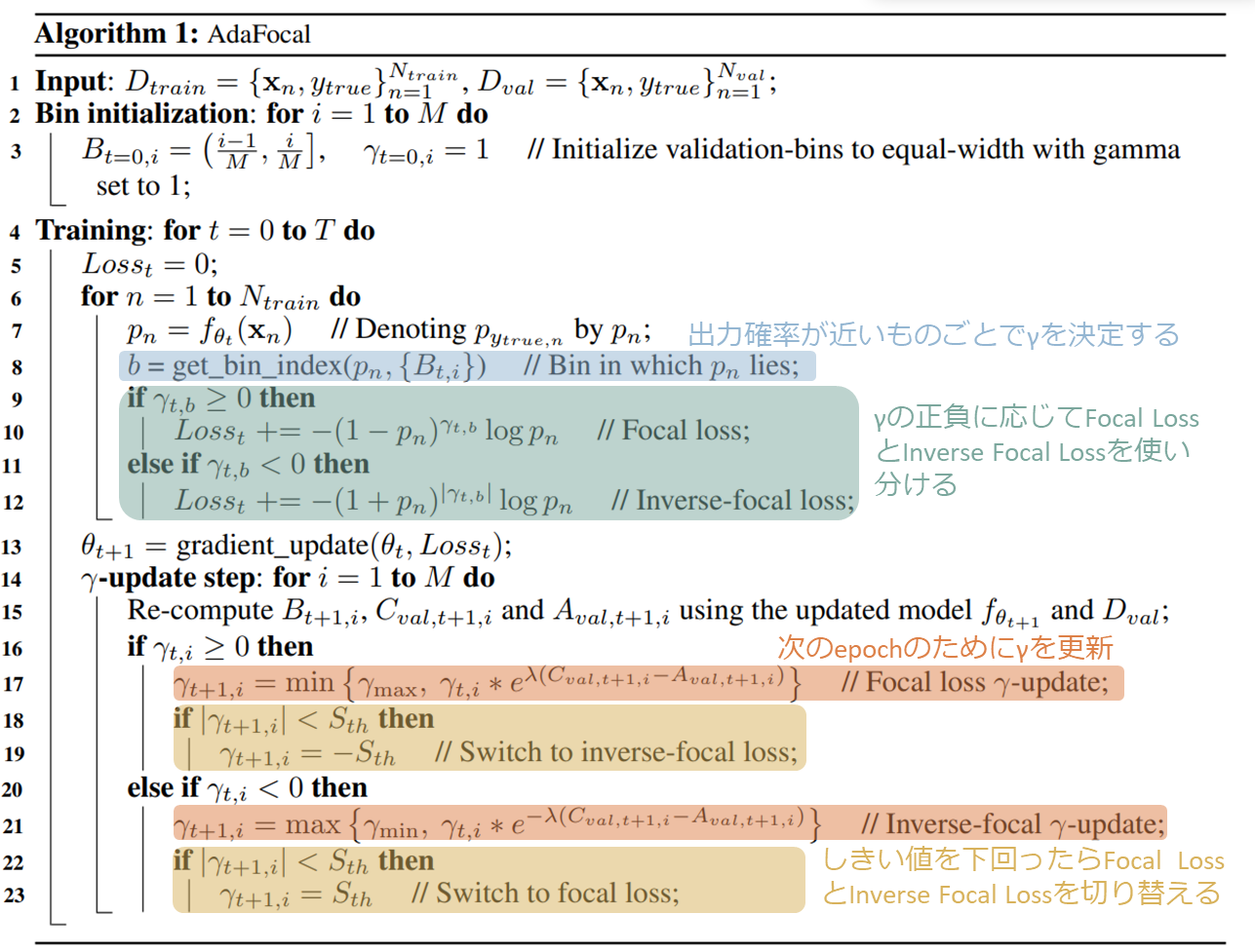
experiment
Verification of Calibration Performance on Classification Problems
We evaluate the performance of the proposed method on image classification (CiFAR-10, CiFAR-100, Tiny-ImageNet, ImageNet) and text classification tasks (20 Newsgroup dataset). ResNet50, ResNet100, Wide-ResNet-26-10, and DenseNet-121 are used for the image classification task, while CNN and BERT are used for the text classification task. In addition to Cross Entropy Loss (CE) and the sample-devpdent focal loss described above (FLSD-53) for the baseline, other calibration learning methods, such as MMCE, Brier loss, and Label smoothing (LS-0. 05) are used as other calibration learning methods and compared with AdaFocal. In addition, comparisons are made with and without temperature scaling.
The results of the evaluation of each method with ECEEM are shown in the table below.
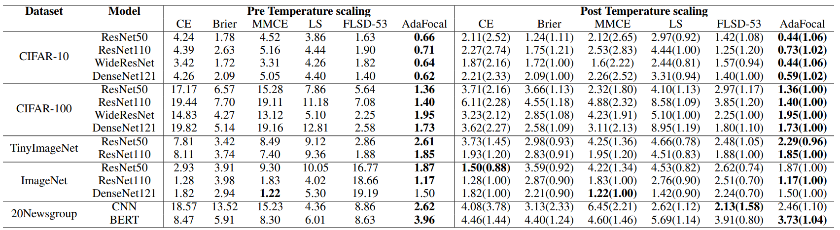
We see that AdaFocal performs best for most data sets, models, and experimental settings.
The following graph visualizes the error rate in classification and the change in ECEEM per epoch.
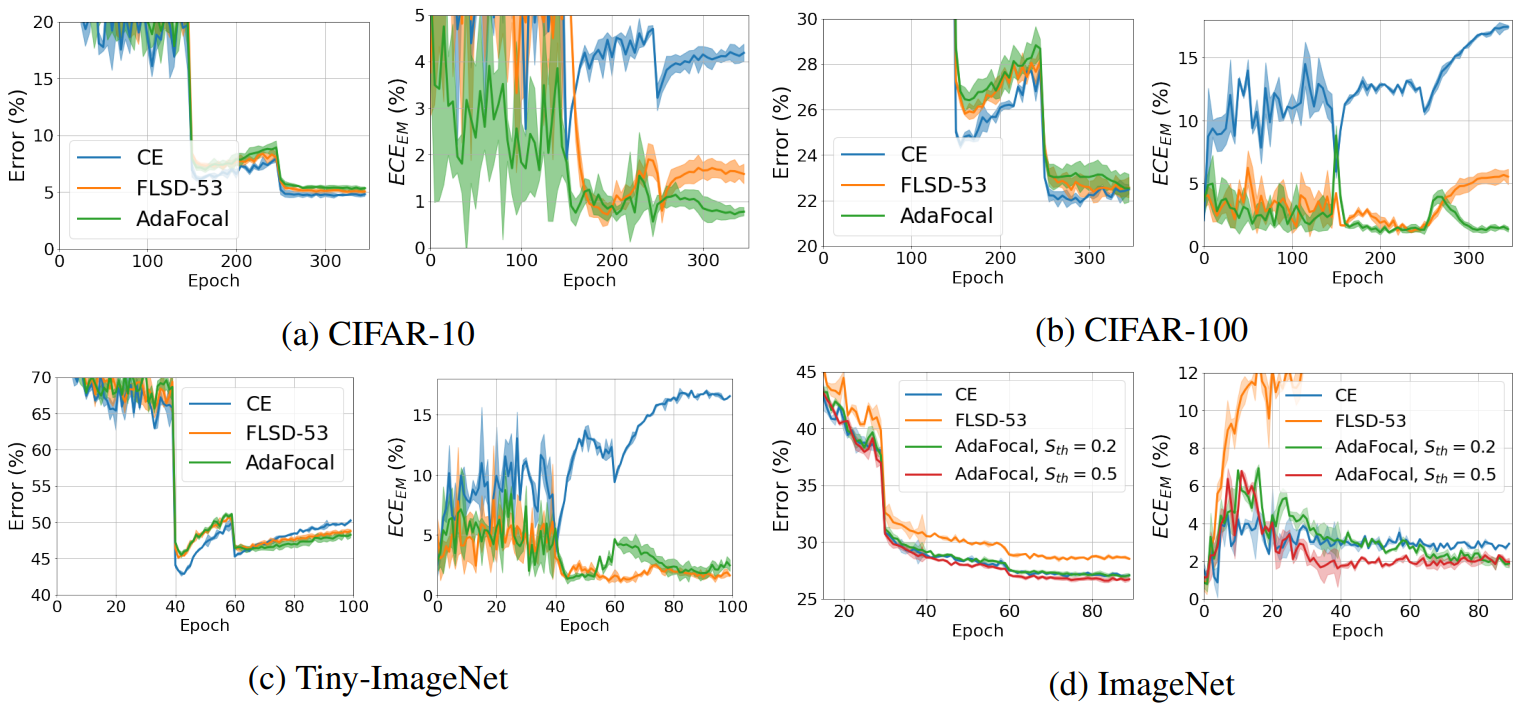
These graphs show that AdaFocal achieves low calibration error while maintaining classification performance comparable to other methods.
Out-of-Distribution detection task
This paper also validates AdaFocal in the Out-of-Distribution (OOD) detection task [6], comparing the results of training with ResNet-110 and WideResNet on a dataset consisting of SVHN and CIFAR-10 plus Gaussian noise. ResNet-110 and WideResNet on a dataset consisting of SVHN and CIFAR-10 plus Gaussian noise. The comparison methods are Focal Loss (γ=3) and FLSD-53. These methods are tested without and with temperature.
The following graph shows the results of the ROC curve.
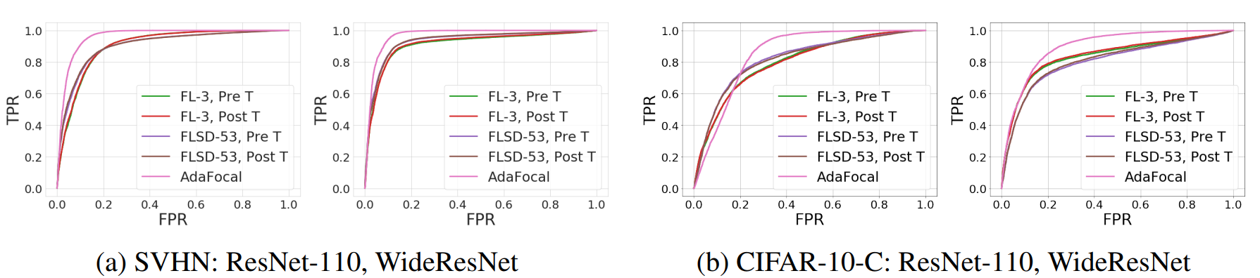
In the ROC curve, a larger area indicates better performance. These graphs show that AdaFocal has the best performance. Therefore, AdaFocal is useful in the OOD detection task.
summary
AdaFocal, an improved version of Focal Loss, was described.
In the classification task, AdaFocal was shown to achieve classification performance comparable to existing methods while improving calibration in many cases.
AdaFocal was also found to be effective in the OOD detection task.
These results suggest that AdaFocal may be useful in improving the explanatory power and reliability of AI.
supplement
[1] In this paper, M=15.
[2] FLSD allows γ to change according to the model's predicted probability in the correct answer label. In this paper, γ = 5 when the model's predicted probability is between 0 and 0.2, and γ = 3 when it is between 0.2 and 1.
[3] In this paper, λ=1 is used because it was confirmed that the accuracy is higher when λ=1.
[4] In this paper, γmin=-2 and γmax=20.
[5] In this paper, Sth=0.2 .
[6]OOD detection task is a task to detect input data not included in the training data, which has been discussed several times in AI-Scholar.
What is the "likelihood ratio" to improve the detection performance of out-of-distribution data?
Ignorance] A New Benchmark and a New Method for Detecting Out-of-Distribution Data that Allows Models to Identify "This is Unknown.


Categories related to this article