Should Unlabeled Data Be Treated As "equal"? A Proposed Method For Extending Semi-supervised Learning

3 main points. 
✔️ Semi-supervised learning after weighting each piece of unlabeled data 
✔️ Automatically weight the data by applying the influenece function 
✔️ Also consider methods that make the proposed method lighter

Not All Unlabeled Data are Equal: Learning to Weight Data in Semi-supervised Learning 
written by Zhongzheng Ren, Raymond A. Yeh, Alexander G. Schwing
(Submitted on 2 Jul 2020 (v1), last revised 29 Oct 2020 (this version, v2))
Comments: NeurIPS camera ready
Subjects: Machine Learning (cs.LG); Computer Vision and Pattern Recognition (cs.CV); Machine Learning (stat.ML)　
 

background

In general, the supervised learning framework requires a large amount of training data, but it is extremely difficult to label each of them by human hands. Semi-supervised learning, on the other hand, is known to be effective in reducing the cost of artificial labeling, because it enables training with some data unlabeled.

Here's a thought: does unlabeled data really contribute to the accuracy of a prediction model? It depends on the learning algorithm, but sometimes unlabeled data can be a hindrance to learning. For example, if you use k-means to fit unlabeled data to a class, there is no guarantee that it is the correct class. Is it OK to train a predictor based on information that is not necessarily correct? It is hard to say to what extent we can trust unlabeled data compared to labeled data.

In this paper, we tackle such a problem and propose a method for semi-supervised learning in which each unlabeled data is given a weight. The idea itself is simple, but we apply a technique called influence function to obtain these weights automatically. The idea is simple, but we apply a technique called influence function to calculate the weights of unlabeled data automatically without our direct intervention. In addition, a simple mechanism is introduced that makes the method proposed in this paper lightweight.

prior knowledge

As a prerequisite, we will briefly introduce the influence function (in this section, we assume supervised learning). influence function is, in a nutshell, a measure of how much a certain data $(x, y)$ influences the learning of a predictor $\theta$. In the following, we will use the labeled training data. In the following, we formulate the influence function $F$ as $\mathcal{D}$ for the set of labeled training data and $\ell_{\text{S}}$ for the loss function.

$F(x, y) = \frac{\partial\theta^{*}(\epsilon)}{\partial\epsilon},$

$where\quad \theta^{*}(\epsilon) := \arg\min\limits_{\theta}\sum\limits_{(x', y')\in\mathcal{D}}\ell_{\text{S}}(x', y', \theta) + \epsilon\ell_{\text{S}}(x, y, \theta)$

However, we set $\epsilon>0$. As shown in the definition above, $\theta^{*}(\epsilon)$ represents the minimizer of the loss $\ell_{\text{S}}(x, y, \theta)$ for some data $(x, y)\in\mathcal{D}$ when up-weighted slightly . The $\epsilon$ can be interpreted as the degree of up-weighting the loss of data $(x, y)$, and by taking the partial derivative of the minimizer, the "degree of influence on learning" is expressed.

However, it is difficult to calculate $\frac{\partial\theta^{*}(\epsilon)}{\partial\epsilon}$ introduced in the above equation on a computer. For this reason, methods to approximate the influence function to a computable form have been actively studied. The following is one such example, which plays a central role in the paper presented here.

$\frac{\partial\theta^{*}(\epsilon)}{\partial\epsilon} = -H_{\theta^{*}}^{-1}\nabla_{\theta}\ell_{\text{S}}(x, y, \theta^{*}),$

$where\quad\theta^{*}:=\arg\min\limits_{\theta}\sum\limits_{(x', y')\in\mathcal{D}}\ell_{\text{S}}(x', y', \theta)$

However, $\ell_{\text{S}}$ is assumed to be second-order differentiable, and $H_{\theta^{*}}$ is the Hessian for $\ell_{\text{S}}$. For a more in-depth understanding of the influence function, the following paper is useful: Understanding black-box predictions via influence functions

proposed method

Before introducing the proposed method, we review semi-supervised learning in general. There are several formulations of semi-supervised learning, and the following is one of them.

$\min\limits_{\theta}\sum\limits_{(x, y)\in\mathcal{D}}\ell_{\text{S}}(x, y, \theta) + \lambda\sum\limits_{u\in\mathcal{U}}\ell_{\text{U}}(u, \theta)$

However, in the above equation, the set of unlabeled training data is $\mathcal{U}$ and the loss function for unlabeled training data is $\ell_{\text{U}}$. The $\lambda$ is a hyperparameter, and the fact that it is out of the sum shows that we have given equal credit to all unlabeled training data. On the other hand, the proposed method in this paper can be formulated as follows.

$\min\limits_{\theta}\sum\limits_{(x, y)\in\mathcal{D}}\ell_{\text{S}}(x, y, \theta) + \sum\limits_{u\in\mathcal{U}}\lambda_{u}\ell_{\text{U}}(u, \theta)$

As before, $\lambda_{U}$ is a hyperparameter, but we can see that it is uniquely assigned to all unlabeled training data. Does this mean that you need to set the hyperparameter manually for each unlabeled training data $\mathcal{U}$? You may think so, but that is not the case. We prepare the test data set $\mathcal{V}$ separately from $\mathcal{D}$ and $\mathcal{U}$, and search for hyperparameters that minimize the loss.

Based on the above, the proposed method optimizes the predictor $\theta$ and the hyperparameter $\Lambda=\{\lambda_{1}, \cdots, \lambda_{|\mathcal{U}|}\}$ by solving the following hierarchical optimization problem.

$\min\limits_{\Lambda}\sum\limits_{(x, y)\in\mathcal{V}}\ell_{\text{S}}(x, y, \theta^{*}(\Lambda)),$

$where\quad\theta^{*}(\Lambda) := \arg\min\limits_{\theta}\sum\limits_{(x, y)\in\mathcal{D}}\ell_{\text{S}}(x, y, \theta) + \sum\limits_{u\in\mathcal{U}}\lambda_{u}\ell_{\text{U}}(u, \theta)$

For later convenience, we will re-formulate it in a different expression.

$\min\limits_{\Lambda}\sum\limits_{(x, y)\in\mathcal{V}}\mathcal{L}_{\text{S}}(\mathcal{V}, \theta^{*}(\Lambda)),$

$where\quad\theta^{*}(\Lambda) := \arg\min\limits_{\theta}\mathcal{L}(\mathcal{D}, \mathcal{U}, \theta,\Lambda )$

In solving the above optimization problem, we need to find the gradient of $\mathcal{L_{\text{S}}}(\mathcal{V}, \theta^{*}(\Lambda))$ for $\lambda_{u}$. This is an inconvenient form to calculate on a computer. In this paper, we use a technique called Danskin's Theorem and the influence function introduced at the beginning of this paper to approximate such a gradient to a computable form.

$\frac{\partial}{\partial\lambda_{u}}\mathcal{L}_{\text{S}}(\mathcal{V}, \theta^{*}(\Lambda)) = \nabla_{\theta}\mathcal{L}_{\text{S}}(\mathcal{V}, \theta^{*})^{\mathtt{T}}\frac{\partial\theta^{*}(\Lambda)}{\partial\lambda_u}\quad$ (Danskin's Theorem)

$=-\nabla_{\theta}\mathcal{L}_{\text{S}}(\mathcal{V}, \theta^{*})^{\mathtt{T}}H_{\theta^{*}}^{-1}\nabla_{\theta}\ell_{\text{U}}(u, \theta^{*})\quad$ (influence function)

However, we defined $H_{\theta^{*}}=\nabla_{\theta}^{2}\mathcal{L}(\mathcal{D}, \mathcal{U}, \theta^{*}, \lambda)$. The influence function is naturally included in the first equation obtained by Danskin's Theorem, which is a neat form. This transformation takes a formulation that is inherently uncomputable on a computer and turns it into a problem of finding the gradient of a loss function, as one would find in a general problem setting.

To solve the proposed optimization problem, we need to find $H_{\theta^{*}}^{-1}$, but the computation of the inverse matrix generally requires a large computational cost. In this paper, as a solution to this problem, only a part of the parameter $\theta$ of the predictor is subject to optimization. Specifically, by tuning only the parameter $\hat{\theta}\subset\theta$ of the final layer of DNN, the number of dimensions is reduced and the inverse matrix calculation is lightened. This is a very drastic method, but later numerical experiments show that it is useful.

numerical experiment

Some of the experiments described in the paper are shown below.

In the first experiment, we use synthetic data of binary classification to show the usefulness of the proposed method. In this experiment, the number of labeled training data is 10 and the number of unlabeled training data is 1,000 (i.e., we assume a situation where the number of unlabeled data is so large that we cannot manually provide hyperparameters $\lambda_{u}$ to each of them). We also assume that the number of test data is 30 and the model is MLP (100 hidden units, ReLU). Now let's move on to the experimental results.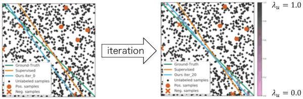

The orange circles and Xs represent positive/negative labeled data, respectively. On the other hand, the black and pink dots represent unlabeled data, which are black as they approach $\lambda_{u}=1.0$ and pink as they approach $\lambda_{u}=0.0$. The green line represents the true decision boundary. The orange line represents the decision boundary when only labeled data is used (supervised learning). Finally, the light blue line represents the decision boundary when both labeled and unlabeled data are used (semi-supervised learning). From the figure, we can see that the light blue line becomes closer to the green line as we turn the iteration, and the color of unlabeled data near the decision boundary becomes closer to pink.

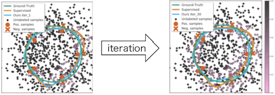
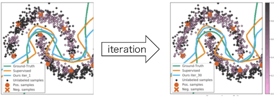
For reference, we also show the results of an experiment using a different synthetic data set.

Next, we present experimental results showing the validity of the approximation method for $H_{\theta^{*}}^{-1}$ introduced in this paper. Although there are other methods to approximate the Hessian, we will compare the accuracy of our method with two of them (Luketina et al., Lorraine et al.). The data set is CIFAR-10 and the prediction model is ResNet.

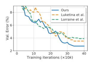
The blue broken line is the proposed method in this paper. The horizontal axis represents the iteration and the vertical axis represents the error on the test data set. From this result, we can see that the Hessian approximation method presented in this paper is more accurate than others.

summary

We introduced a method that extends semi-supervised learning to automatically weight each unlabeled data. The idea of the method itself is very simple, but by introducing Danskin's Theorem and the influence function, we have reduced it to a computationally tractable formulation. Since there has been a lot of research on labeling cost reduction for a long time, it would be interesting to analyze the relationship and combination with other methods.

Categories related to this article

• Article
• Machine Learning