VoxelMorph: A UNet-based Registration Model For Medical Imaging!
3 main points
✔️ Costly optimization solved for each image pair is replaced by a single global optimization
✔️ Works overwhelmingly fast with the same accuracy as conventional methods
✔️ Flexible model that can improve accuracy if each image has partial auxiliary data
VoxelMorph: A Learning Framework for Deformable Medical Image Registration
written by Guha Balakrishnan, Amy Zhao, Mert R. Sabuncu, John Guttag, Adrian V. Dalca
(Submitted on 14 Sep 2018 (v1), last revised 1 Sep 2019 (this version, v3))
Comments: Published on arxiv.
Subjects: Computer Vision and Pattern Recognition (cs.CV)
code:

The images used in this article are from the paper, the introductory slides, or were created based on them.
first of all
We present a model for non-rigid registration (DIR) called VoxelMorph, which was proposed in 2018. The registration task, also known as alignment, has the purpose of capturing the correspondence between images in which an object or region is moving. In the medical field, this task is expected to be applied to MRI and CT image pairs. For example, it can be used in lung CT image pairs where tissue movement is observed due to breathing, or in MRI images to compare symptoms of a target area between patients.
The correspondence can be found by obtaining the displacement field, which represents how each part has moved or deformed between images. before VoxelMorph was published in 2018, DIR was mainly used to optimize each image pair separately. Instead of deep learning models that learn parameters such that a single model maps the entire dataset, non-training-based methods such as the Demons algorithm that solves the optimization problem for each image set achieved high accuracy. VoxelMorph formulated the DIR task as a parametric function that takes a set of images as input and outputs a displacement field. In other words, VoxelMorph's process is completed by the following simple equation
While most deep models require a single image as input(although mini-batching is performed ), VoxelMorph requires a set of images as input, thus allowing us to build a model that can globally learn and optimize the parameter θ across the entire dataset, rather than optimizing each image set separately. This allows us to build a model that can learn and optimize the theparameterθglobally across the entire dataset, rather than optimizing each image pair separately. f is the target image to transform (fixed) and m is the reference image to transform (moving).
VoxelMorph is a well-known learning-based DIR model, but there are not many articles about it in Japanese. The main advantages of VoxelMorph are as follows.
- A deep learning model that performs global optimization on the entire dataset
- Can be trained on small data sets
- Overwhelmingly fast with the same accuracy as conventional methods
- By using U-Net, we can learn to capture the exact location of features
- Supervised loss can be added if auxiliary data is available for each image
- Support for both 2D and 3D images
The experiments analyze the effect of appearance loss, the presence of auxiliary data, and their weight settings on the accuracy, as well as the effect of accuracy on the size of the dataset. Let's quickly look at the details of VoxelMorph. *This explanation is based on the technology in 2018,19 at the time of publication of the paper.
systematic positioning
First, we explain the systematic position of this method. Transformations handled by the registration task are largely divided into rigid and non-rigid transformations. Rigid registration handles affine transformations in which the shape of the object or region in the image does not change and only translations and rotations are observed. In contrast, most medical images are non-rigid registration (DIR). Tissues in the body move more freely than we think, and many non-linear deformations change shape in response to breathing and body movements, and the images vary from subject to subject.
However, DIR may also perform affine and non-linear transformations in two steps. VoxelMorph focuses on the second step in the DIR task, which is to reduce the overall shift and rotation of the image by affine transformations. The VoxelMorph is focused on the second step in the DIR task and targets image pairs in which the overall shift or rotation of the image has been reduced by an affine transformation.
architecture
The architecture of VoxelMorph is shown in the figure below.
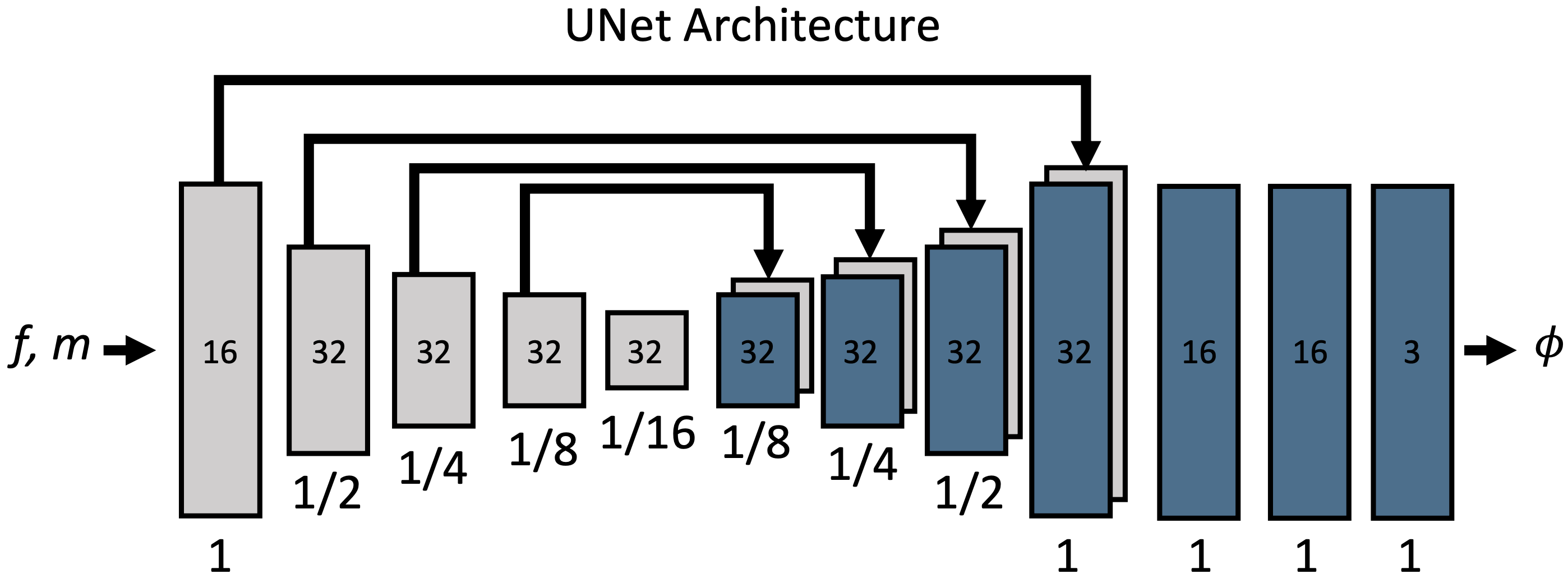
Φrefers to the displacement field. Φ and f,m are of the same size. We can see that we have realized g(f,m)=u, which takes an image pair as input and outputs a displacement vector. The number in the block is the number of channels, and below it is the scale concerning the input size. The detailed settings are shown below.
- The implementation simply treats it as an image with 2 channels
- The figure shows an example of a 3D image, so the output displacement field has three channels
- Each convolution layer defaults to a 3x3 kernel and stride 2, but it is argued that this should be changed to match the size of the displacement assumed for the CNN
- After each convolution layer, a LeakyReLU with α=0.2 is applied
But why does this mechanism successfully learn the parameter θ that outputs the displacement field between images? The key lies in UNet.
UNet
Although we can assume multidimensional output even in a general regression task, in this task we need to output g(f,m)=u. That is, if the image size is 256x256, the output must be 256x256x2D, considering 2-D migration, and must exhaustively capture the deformation for each voxel.
However, CNN assumes the locality of features and captures global features as the layer gets deeper. In this case, no matter how good the Decoder is, the position of features becomes ambiguous as the depth of the layer increases, and the accurate displacement field can no longer be output. This is where UNet comes into play.
UNet is a neural net consisting of an Encoder and a Decoder, Encoder consists of convolution and Max-pooling, Decoder consists of convolution and Upsampling. Here, instead of just connecting them directly, we perform Skip-Connection, which keeps the Encoder's feature map and connects it to the Decoder's feature map of the same size. By doing this, the localized low-level features captured by the Encoder can be output together with the refined features of the Decoder, and a feature map that maintains accurate location information and feature quality can be obtained. Because its connection looks like a U shape (you can't see it in the above figure...) It is called UNet.
UNet is mainly used in segmentation tasks, but VoxelMorph applies its advantage to DIR. It outputs a displacement field based on features of various granularities extracted from a reference image m and a target image f, respectively, with several additional layers of convolution.
Spatial Transformer Networks(STN)
VoxelMorph outputs the displacement field, but to evaluate the accuracy of the displacement field, we need to transform m based on the displacement field and evaluate whether it matches f. VoxelMorph uses a Spatial Transformer (STN), which is different from the familiar Transformer used in Attention. VoxelMorph uses a Spatial Transformer (STN), which is different from the familiar Transformer in Attention, and simply transforms the space based on the displacement field. For a voxel p, we transform it as follows.
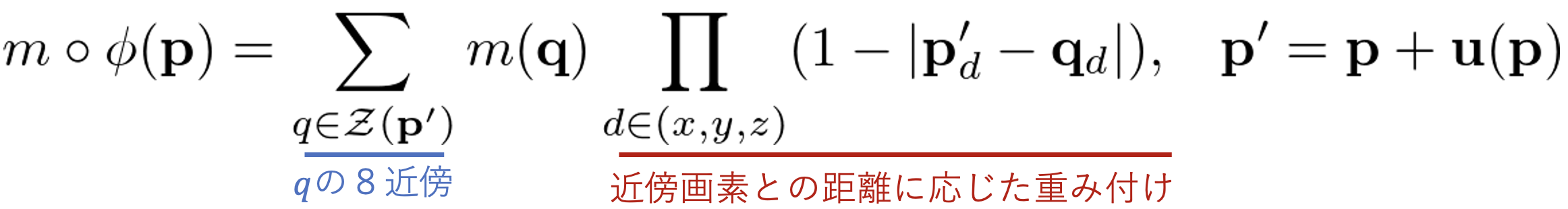
As shown in the equation, the process is not deforming m, but rather assigning the value of the deformed voxel p' to the value of voxel p. Since p' cannot be directly referenced, it is weighted by the nearest neighbor pixel q in the 8 directions. In this case, p' cannot be directly referenced, so the weighting is done by the nearest neighbor pixel q in the 8 directions. u output by VoxelMorph is not necessarily an integer, so it is necessary to interpolate by the nearest neighbor pixel if the pixel is located between pixels. |If q happens to be an integer, the weight is 1 for the center coordinate and 0 for the others, otherwise it is weighted and added according to the distance.
After transforming m by STN according to the displacement vector estimated in this way, the loss and evaluation are taken.
loss function
There are two types of loss functions in VoxelMorph, supervised and unsupervised, for each image. Unsupervised loss is accurate enough, but if each image has segmentation data showing anatomical structures, the accuracy can be improved by adding supervised loss to impose their matching.
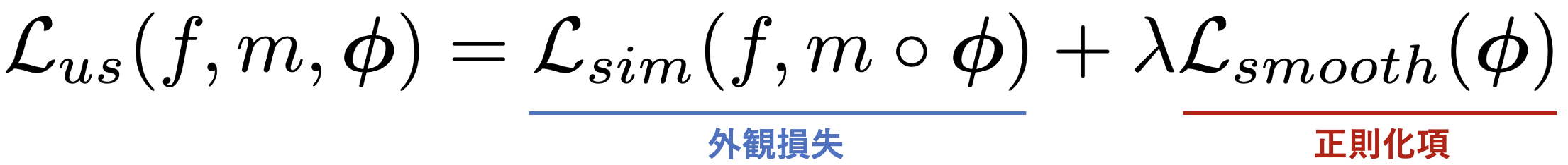
unsupervised loss
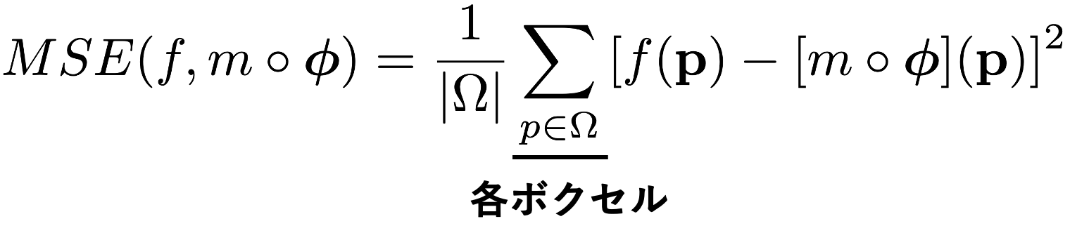
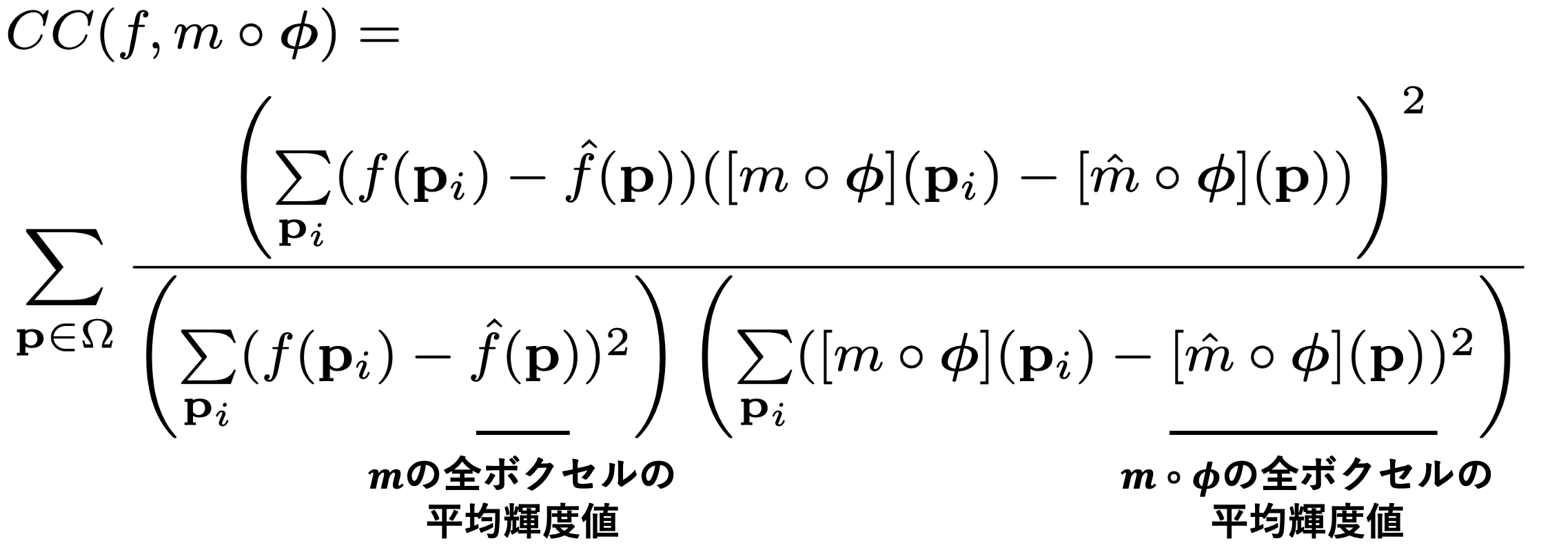
Unsupervised loss is a common loss in DIR. It consists of an apparent loss that imposes a visual match between the transformed image pairs and a regularization term that suppresses local changes in the displacement vector. The appearance loss can be any differentiable error function, and in the paper, we use MSE (Mean Squared Error) and NCC (Normalized Cross Correlation) Loss. MSE is a simple pixel-to-pixel squared error, while NCC is a robust measure for differences in luminance values that are not related to the structure of the region.
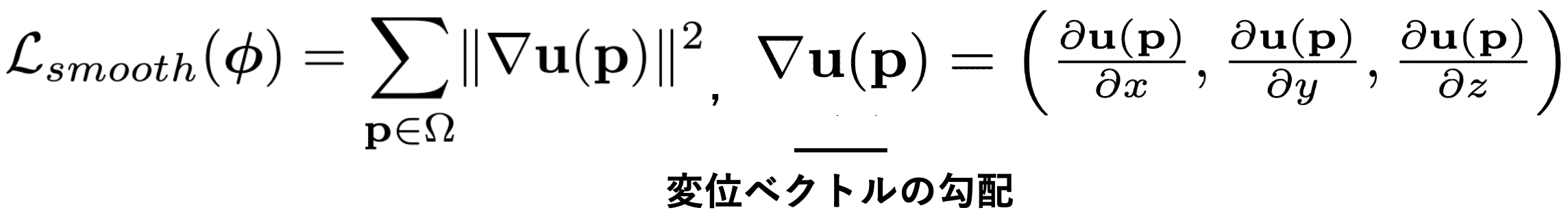
However, this alone does not output unnatural vectors that force the appearance to match. As long as we are dealing with real-world images, it is natural for vectors to have the same magnitude and flow in the same direction in local areas. Experiments have confirmed that such regularization is more accurate. The regularization term is expressed by the following equation, where the magnitude of the gradient of u is the loss, which suppresses abrupt local changes in the vector.
supervised loss
If segmentation data representing anatomical structures are present, we take not only appearance loss but also structure match as a loss. The Dice coefficient is a measure of the overlap between the two masks. When there are K segmentation data in an image pair, the loss is expressed as
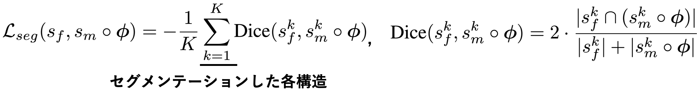
This can be weighted and added to the unsupervised loss to improve accuracy. In this case, we have two weights as hyperparameters: λ for the constraint term and γ for the supervised loss.
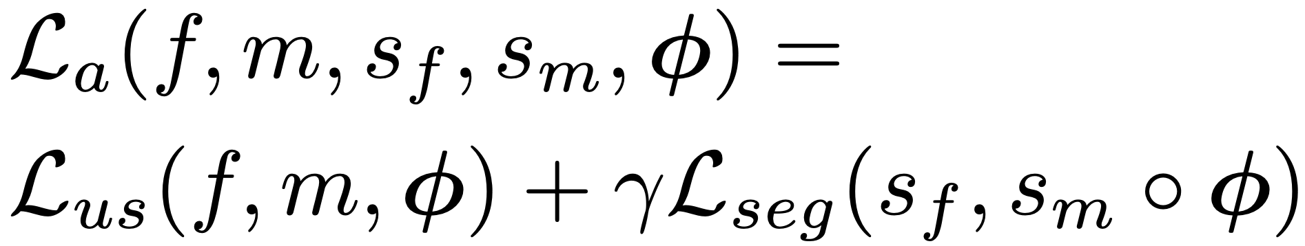
VoxelMorph performs global optimization by taking these structures and losses.
experiment
Experiments test the accuracy of the VoxelMorph under various settings of the loss selection and weights described earlier. In all experiments, we assume that a linear deformation is captured by an affine transformation in the first step. We have performed a variety of analyses, but here we only show a few representative experiments.
setting (of a computer or file, etc.)
comparative approach
The comparison method employs Symmetric Normalization (SyN), which was state-of-the-art in 2019, andNiftyReg, free software that performs DIR.SyN seems to be a method to find the displacement field that maximizes the cross-correlation between images using Eulerian-Lagrangian equations. NiftyReg seems to capture affine deformations in the first step and nonlinear deformations by free-form-deformation (FFD) in the second step.
VoxelMorph is trained using Adam, but with a batch size of 1.
data-set
The experiments are performed on 3,731 head MRI (T1-weighted) images of eight datasets. To validate the auxiliary data, segmentation data were obtained for each dataset using the tool FreeSurfer (see below) and affine transformations were applied. data, which is completely unknown and only used for testing purposes to validate the accuracy of the We use the obtained segmentation data for 30 different anatomical structures, partitioned by Train:Valid: Test=3231:250:250.
valuation index
The evaluation is based on the Dice score of the segmentation map created above. Apart from that, we also use the Jacobi matrix to evaluate whether we have generated natural vectors or not. If the Jacobi matrix is positive, it can be regarded as a diffeomorphism, which means that the displacement field is smooth. Here, we count the number of voxels whose Jacobi matrix is less than or equal to zero and use it as an indicator to evaluate the displacement field. The Jacobi matrix is expressed as
![]()
Accuracy verification of unsupervised loss
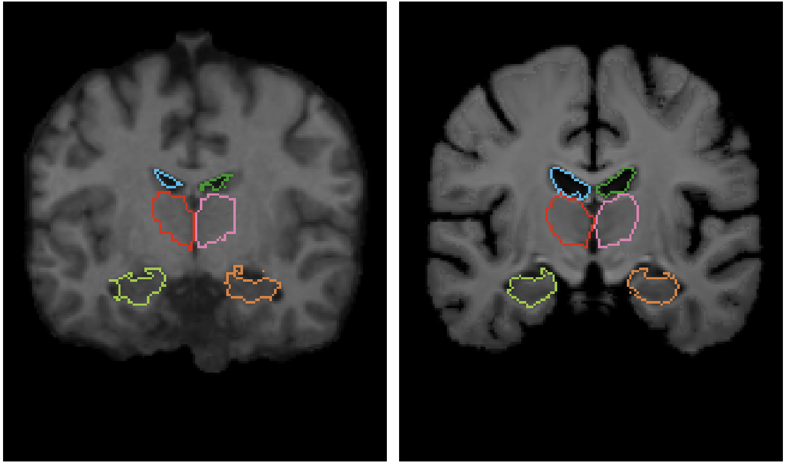
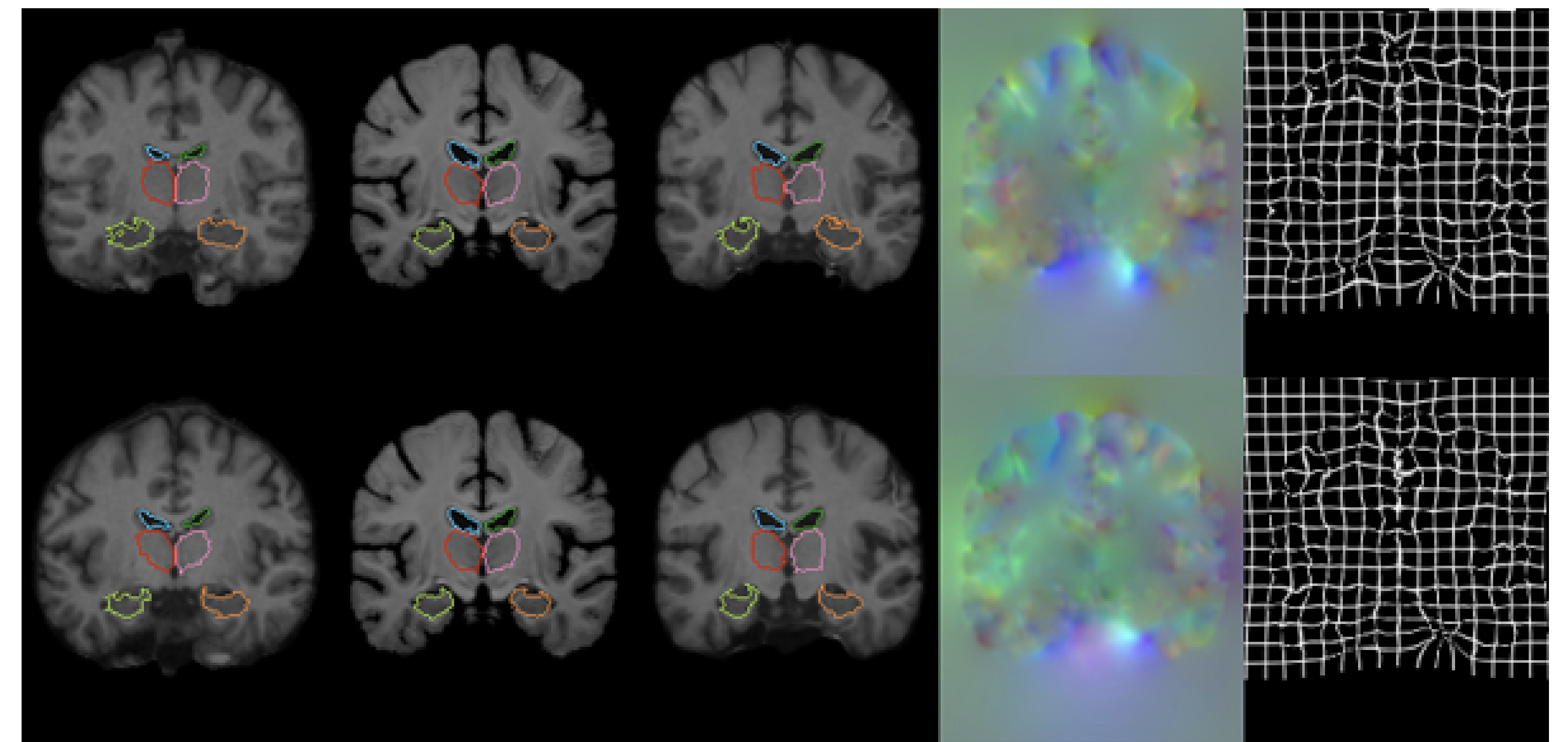
Results for the full data set are shown. In parentheses are the standard deviations. From top to bottom: affine transform only, existing methods (both using CC), and VoxelMorph (CC and MSE). The application examples are further illustrated in the figure below, where VoxelMorph improves the accuracy over the affine transform and achieves a Dice score comparable to SyN and NiftyReg. The CPU speeds of VoxelMorph are significantly faster than SyN and NiftyReg: VoxelMorph is about 150 times faster than SyN and about 40 times faster than NiftyReg. This is because the existing methods perform optimization for each image pair, and the execution time varies greatly depending on the degree of deformation of the data. The GPU version of VoxelMorph was not publicly disclosed, so comparisons could not be made.
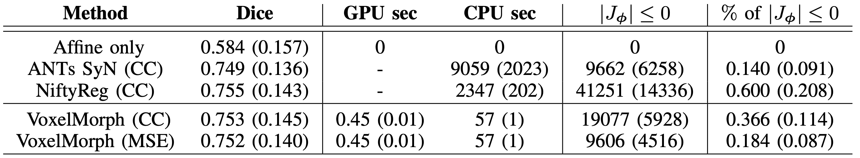
The number of voxels with Jacobi matrix less than zero is shown, and the applied results show that the regularization term works well to generate a smooth displacement field.
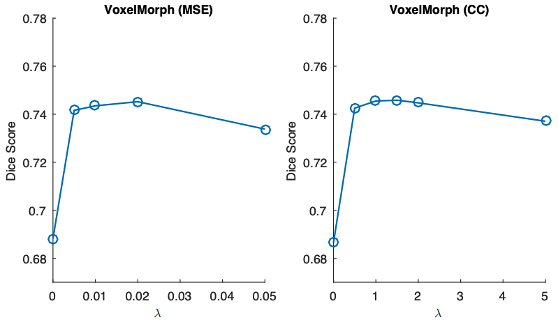
Sensitivity analysis for the weights λ of the regularization terms
Here we analyze the variation of the Dice coefficients for different values of λ. First of all, we can see that the regularization improves the accuracy compared to the case of appearance loss alone (λ=0). We can also see that the variation is robust and less sensitive to the choice of λ for both MSE and CC.
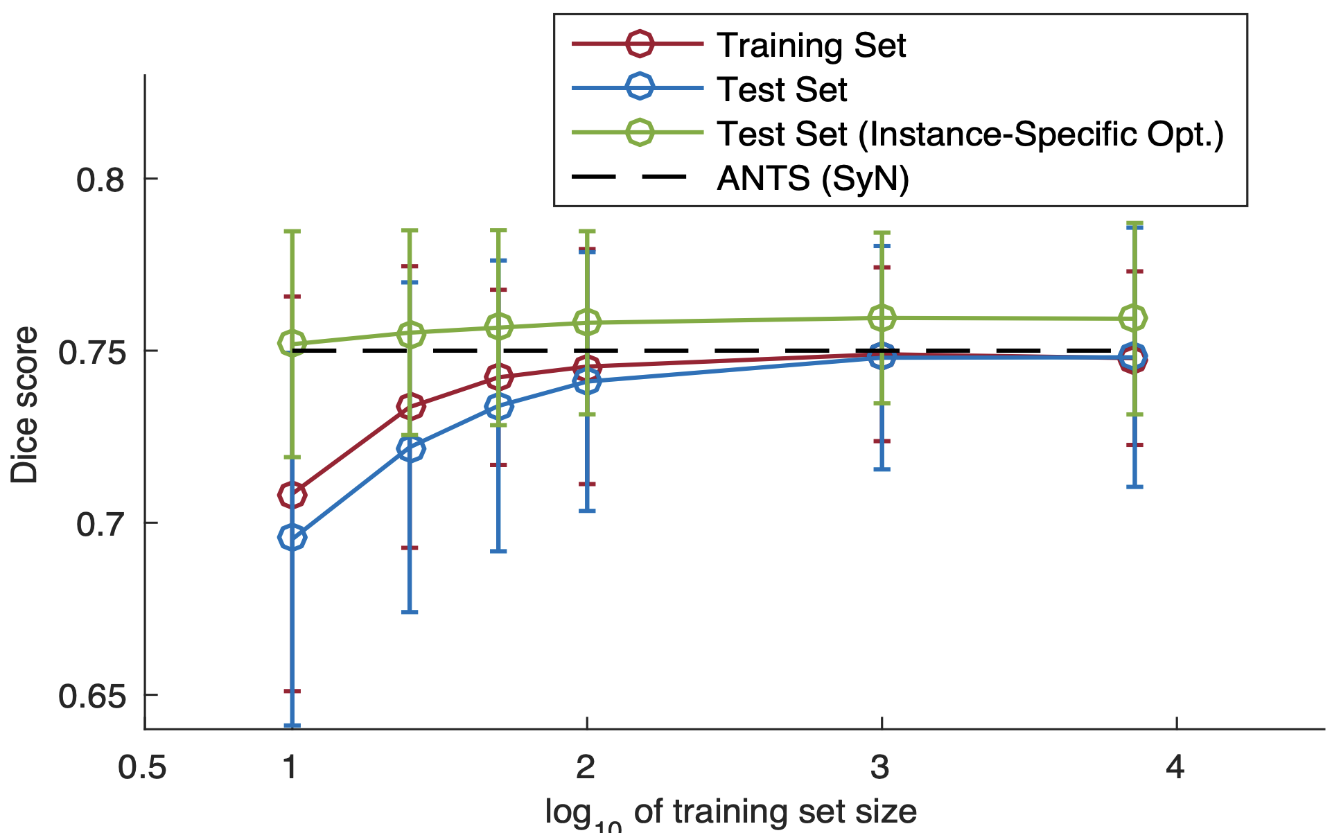
Analysis of dataset size and individual optimization
The second issue is the effect of the size of the dataset on the optimization: even though only one global optimization is needed, the range of applications is limited if the dataset is too large. In this experiment, we analyze the change in accuracy when the data used for training is varied from 10, 100, 1000, and 10000. The horizontal axis of the table is the logarithm of the normal logarithm. The dashed line shows SyN as a comparison. If there are only 10 pairs of data, the accuracy is too small, but if there are 100 pairs of data, the Dice coefficient is more than that and it is almost the same, so you can see that the accuracy is almost the same. The green line shows the accuracy of training on the test data individually, and the results show that after the global optimization of VoxelMorph, the accuracy improves, even more, when the data is optimized individually, as it has been done before. In this case, the size of the dataset does not matter much.
Accuracy verification of supervised loss
Then we compare the accuracy when adding supervised loss using auxiliary data. We use MSE with λ=0.02 here because both MSE and CC had similar accuracy with unsupervised loss. Four patterns are assumed for the auxiliary segmentation data. Segmentation data is a heavy burden to annotate, and it is unrealistic to assume that convenient data is always available. Therefore, we assume three patterns when only a part of the 30 anatomical segmentations created are obtained, and one pattern when the segmentation data is rough.
- One Observed: Data was obtained for only one type of structure among "hippocampus, cerebral cortex, white matter, and ventricles".
- Half Observed: 15 random data from 30 different structures
- All: Data for which all structures have been obtained
- Coarse Segmentation: data from 30 fine annotations divided into 4 rough segmentations: white matter, gray matter, cerebrospinal fluid, and brainstem
Patterns 1 to 3 analyze the effect of the amount of segmentation, while pattern 4 analyzes the effect of segmentation roughness on the fine structure estimation system. The accuracy for the seven datasets annotated with FreeSurfer (FS), the accuracy for The following figure shows the accuracy for the seven datasets annotated by FreeSurfer(FS) and the accuracy for the manually annotated Buckner40.
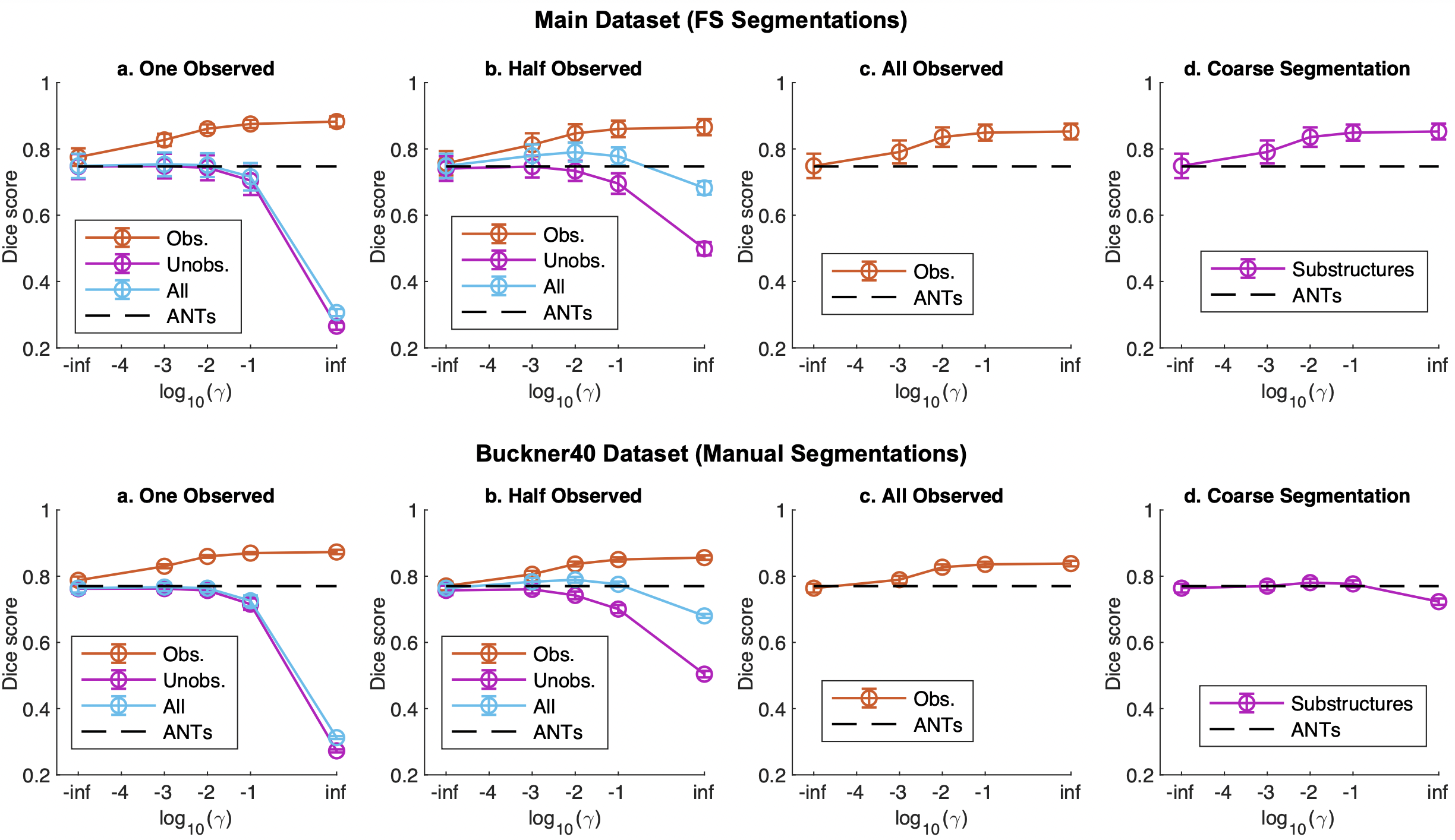 Since the abscissa is logarithmic, -inf means unsupervised loss, and inf means only supervised loss; too large a value of γ will overtrain the Observed and reduce the accuracy of the Unobserved, but a moderate adjustment will outperform the unsupervised loss, and ANTs(SyN ). The All Observed, where all the structure is available, gives higher accuracy, but most importantly, there is also a contribution from the Unobserved data, where the structure is not available. Buckner40 has a similar trend, but the increase in Coarse Segmentation seems to be smaller because the Dice score is higher.
the others
We are also searching for parameters that are compatible with λ and γ, and comparing the accuracy of each site. If you are interested, please refer to the paper.
impression
Appearance loss seems to be worth trying different things; SSIM Loss seems to behave differently from MSE because it captures differences on a domain basis from three perspectives: luminance value, variance, and structure.
I was curious about the effectiveness of affine transformations. I was focusing on the processing after applying the affine transformation in the first step. Still, I'm curious how effective it is when processing end-to-end without applying the affine transformation. I applied it to MNIST at hand, and it was able to handle quite large affine transformations.
summary
The UNet-based DIR model VoxelMorph was explained.VoxelMorph is as accurate and fast as conventional methods, can be trained on a small data set, is highly flexible, and can be further improved with auxiliary data. It is also claimed that
- In the experiment, only one type of auxiliary data was tested, but it works even when the modality is different, and various types of auxiliary data such as feature points can be used instead of segmentation.
- VoxelMorph is versatile and useful for other registries such as cardiac MRI and lung CT
This model is from 2019, but an improved method called VoxelMorph++ has recently been proposed; GAN-based methods are also strong in DIR, but it is still a practical method with the potential for faster processing.


Categories related to this article

![DrHouse] Diagnostic](https://aisholar.s3.ap-northeast-1.amazonaws.com/media/February2025/drhouse-520x300.png)
![SA-FedLoRA] Communic](https://aisholar.s3.ap-northeast-1.amazonaws.com/media/October2024/sa-fedlora-520x300.png)

![[SpliceBERT] A BERT](https://aisholar.s3.ap-northeast-1.amazonaws.com/media/July2024/splicebert-520x300.png)
![[IGModel] Methodolog](https://aisholar.s3.ap-northeast-1.amazonaws.com/media/July2024/igmodel-520x300.png)