
New Semi-supervised Segmentation: Contrastive-consistent Learning
3 main points
✔️ We developed the first semi-supervised segmentation framework that considers both the consistency property and the contrastive property of a pixel.
✔️ Extended existing image-level contrastive learning to the pixel level. In particular, we used a novel negative sampling technique to reduce the computational cost and false negative rate.
✔️ Recorded SOTA in existing benchmark experiments.
Pixel Contrastive-Consistent Semi-Supervised Semantic Segmentation
written by Yuanyi Zhong, Bodi Yuan, Hong Wu, Zhiqiang Yuan, Jian Peng, Yu-Xiong Wang
(Submitted on 20 Aug 2021)
Comments: ICCV 2021
Subjects: Computer Vision and Pattern Recognition (cs.CV)
code:
The images used in this article are from the paper, the introductory slides, or were created based on them.
first of all
Today's semantic segmentation using deep learning requires a large amount of label data, and the performance degrades significantly when the label data is reduced. However, generating a huge amount of label data is expensive, and semi-supervised learning, which maintains performance with a small amount of label data, is attracting attention. In this paper, we proposed a semi-supervised learning model with two properties to be satisfied: one is called the consistency property in the label space, which indicates that the segmentation result does not change when the object color is changed. The other is called the contrastive property in the feature space, which indicates that the features of the model can group similar pixels into the same group and dissimilar pixels into different groups. Conventional semi-supervised learning SOTA models consider the above-mentioned consistency property, but the contrastive property has not been considered much. In this paper, we proposed a pixel-contrastive-consistent semi-supervised segmentation method (${\rm PC^2Seg}$) that considers both properties.
technique
The schematic diagram of the method is shown in the figure below.
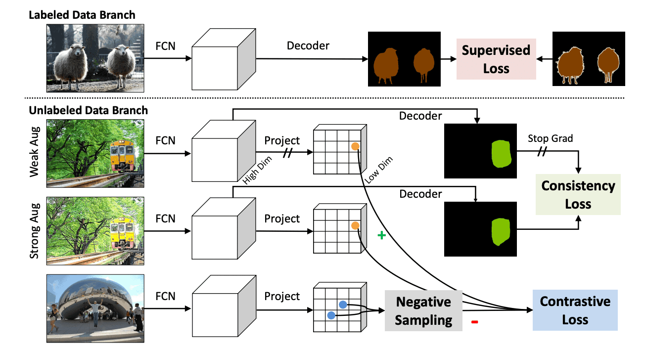
The loss function of ${\rm PC^2Seg}$ is the sum of the loss functions of the labeled and unlabeled data and is expressed as
$${\cal L}={\cal L}^{label}(x,y)+{\cal L}^{unlabel}(x)$$
However, $x$ is the image and $y$ is the mask image. The loss function for labeled data was computed using ordinary cross entropy. The loss function for unlabeled data was computed in a Siamese network architecture using data multiplied by a strong and weak augmentation. Finally, using the consistency loss $l^{cy}$ and the contrastive loss $l^{ce}$, it is expressed as
$${\cal L}^{unlabel}=\sum_{i}\lambda_1 l^{ce}(z_i,z_i^+, \{z_{in}^-\}_{n=1}^N)+\lambda_2 l^{cy}({\hat {\bf y}}_i, {\hat {\bf y}_i^+})$$
where $i$ is the index of the pixel, $z_i$ is the anchor pixel of the weakly augmented image, $z_i^+$ is the positive pixel of the strongly augmented image, $z_{in}^-$ is the negative pixel, ${\hat {\bf y}}_i, {\hat {\bf y}_i^+}$ are the respective predicted probability of the model. Also, $\lambda$ is the balance parameter.
Consistency loss
The consistency loss $L_I^{cy}$ is defined as
$$l_i^{cy}=1-\cos({\hat {\bf y}_i}, {\hat {\bf y}_i^+})$$
where $\cos({\bf u}, {\bf v})=\frac{{\bf u}^T{\bf v}}{|||{\bf u}||_2|||{\bf v}||_2}$ is the cosine similarity. We also introduced gradient stops in the weakly augmented images and backpropagation in the strongly augmented images.
Contrastive loss
The contrastive loss$l_i^{ce}$ is defined as
$$l_i^{ce}=-\log{\frac{e^{\cos({\bf z}_i,{\bf z}_i^+)/\tau}}{e^{\cos({\bf z}_i,{\bf z}_i^+)/\tau}+\sum_{n=1}^Ne^{\cos({\bf z}_i,{\bf z}_{in}^-)/\tau}}}$$
where ${\bf z}_i\in {\mathbb R}^D$ is a $D$-dimensional feature vector and $\tau$ is a temperature parameter.
However, there are some problems in optimizing the above equation. First, the feature vectors are high dimensional and thus computationally expensive. So, we reduce the dimension to low by adding a linear mapping layer. Also, since we are looking at every pixel, the number of negative samples is huge and the noise effect on wrong negative samples is large. Therefore, we used a new sampling method.
Negative Sampling Method
Suppose that for every $i$-th anchor pixel, $N$ negative pixels $z^-_{in}$ follow the following discrete probability distribution.
$$z_{in}^-\sim Discrete(\{z_j\}_{j=1}^M;\{p_{ij}\}_{j=1}^M)$$
For $\{P_{IJ}C}$, we considered the following four methods.
uniform
Simply sample from all pixels $M$ except the anchors in the mini-batch. However, since many pixels in the same image belong to the same category, we take many false negatives.
$$p_{ij}=\frac{1}{M}$$
Different Image
To reduce false negatives, a sample from an image different from the anchor. Let $I_i, I_j$ be the anchor and the ID of the candidate image for the negative sample.
$$p_{ij}=\frac{{\bf 1}\{I_i\neq I_j\}}{\sum_{k=1}^M{\bf 1}\{I_i\neq I_k\}}$$
Pseudo-Label Debiased
Let ${\hat y}_i, {\hat y}_j$ be the predicted labels of pixels $i,j$ respectively. Sample these as pseudo labels from pixels that are predicted to be in a different class than the anchor.
$$p_{ij}=\frac{P({\hat y}_i\neq{\hat y}_j)}{\sum_{k=1}^MP({\hat y}_i\neq{\hat y}_k)}=\frac{1-{\vec{\bf y}_i^T}{\vec{\bf y}_j}}{\sum_{k=1}^M1-{\vec{\bf y}_i^T}{\vec{\bf y}_k}}$$
Different Image + Pseudo-Label Debiased
The combination of the above two methods can reduce false negatives more.
$$p_{ij}=\frac{{\bf 1}\{I_i\neq I_j\}\cdot (1-\vec{{\bf y}}_i^T\vec{{\bf y}}_j)}{\sum_{k=1}^M{\bf 1}\{I_i\neq I_k\}\cdot(1-{\vec{{\bf y}}_i^T}{\\vec{{\bf y}}_j})}$$
This method was used in this paper.
result
We evaluated the performance against the public datasets VOC 2012, Cityscapes, and COCO. The results are shown in the table below.
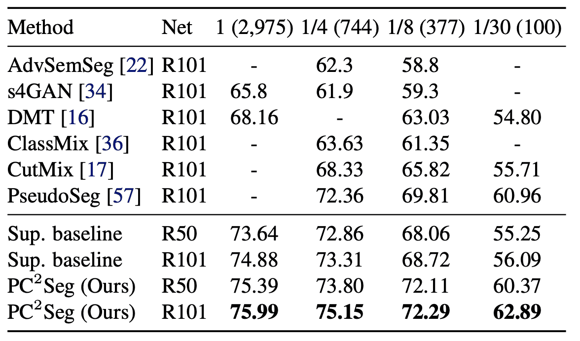
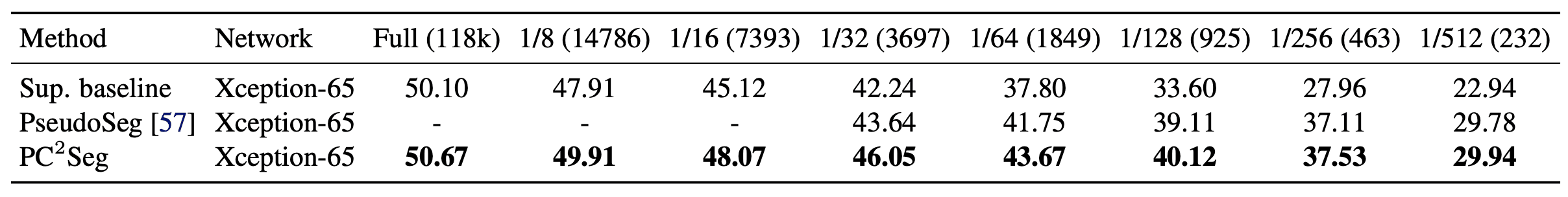
Here the $1/N$ column uses only $1/N$ of the total label data. From the table, we can see that this method ($PC^2Seg$) records SOTA for all datasets. In particular, for Cityscapes, the difference is only 0.84% between using the whole data and using 1/4 of the data. ResNet50 also shows comparable performance to ResNet101, suggesting that the architecture does not need to be that deep with small amounts of data.
summary
In this paper, we proposed a new semi-supervised segmentation method called pixel-contrastive-consistent learning. We also used a new negative sampling method to efficiently learn the contrastive loss. The proposed method outperformed SOTA on existing benchmarks and was found to be a promising method to improve semi-supervised segmentation.


Categories related to this article