Understanding The Behavior Of Contrastive Loss

Contrastive Learning 01/11/2021

3 main points
✔️ Analyze Contrastive Loss used for contrastive learning
✔️ Analyze the role of temperature parameters in Contrastive Loss
✔️ Examine the importance of the Hardness-aware property in Contrastive Loss

Understanding the Behaviour of Contrastive Loss
written by Feng Wang, Huaping Liu
(Submitted on 15 Dec 2020 (v1), last revised 20 Mar 2021 (this version, v2))
Comments: Accepted to CVPR2021.
Subjects: Machine Learning (cs.LG)

code：

The images used in this article are from the paper, the introductory slides, or were created based on them.

first of all

SimCLR, MoCo, and other representation learning methods that use contrastive learning (Contrastive Learning) have been used with excellent success.

In the paper presented in this article, we analyzed various aspects of Contrastive Loss used in contrast learning, including the effect of the temperature parameter $\tau$. Let's take a look at them below.

Analysis of Contrastive Loss

About Contrastive Loss

Initially, for the unlabeled training set $X=\{x_1,...,x_N\}$, the Contrastive Loss is given by the following equation.

$L(x_i)=-log[\frac{exp(s_{i,i/\tau})}{\sum_{k \neq i}exp(s_{i,k}/\tau)+exp(s_{i,i}/\tau)}]$

Where $s_{i,j}=f(x_i)^Tg(s_j)$ is the similarity, $f(\cdot)$ is the feature extractor that maps the image to the hypersphere, and $g(\cdot)$ is some function (identical to $f$, memory bank, momentum queue, etc. ). $\tau$ is a temperature parameter.

In this case, the probability that $x_i$ is recognized as $x_j$, $P_{i,j}$ (the probability that $x_i$ and $x_j$ are considered to be positive samples of each other), can be defined as follows.

$P_{i,j}=\frac{exp(s_{i,j}/\tau)}{\sum_{k \neq i}exp(s_{i,k}/\tau)+exp(s_{i,j}/\tau)}$

Contrastive loss aims to separate the representations of positive samples (e.g., the same image with different transformations) from their neighbors, and the representations of negative samples (different source images) from their neighbors.

In other words, we aim to make the similarity $s_{i, i}$ of the representations between positive samples large and the similarity $s_{i,k}, k\neq i$ of the representations between negative samples small.

Gradient Analysis

Next, we analyze the gradients for the positive and negative samples. Specifically, the gradient for the similarity $s_{i,i}$ between positive samples and the gradient for the similarity $s_{i,j}(j \neq i)$ between negative samples are expressed as follows.

$\frac{\partial L(x_i)}{\partial s_{i,i}}=-\frac{1}{\tau}sum_{k \neq i}P_{i,k}$

$\frac{\partial L(x_i)}{\partial s_{i,j}}=\frac{1}{\tau}P_{i,j}$.

From these equations, we see that

The gradient for negative samples is proportional to exp(s_{i,j}/\tau), and the magnitude of the gradient varies with the values of similarity $s_{i,j}$ and temperature $\tau$.
The magnitude of the gradient for the positive samples is equal to the sum of the gradients for all the negative samples ($\sum_{k\neq i}|\frac{\partial L(x_i)}{\partial s_{i,k}}|/|\frac{\partial L(s_i)}{\ partial s_{i,i}}|=1$).

Analysis of the role of temperature $\tau$.

In conclusion, the temperature $\tau$ serves to control the strength of the penalty (magnitude of the gradient) for negative samples with high similarity of representation ($s_{i,k}(k \neq i)$ is large).

First, for $r_i(s_{i,j})=|\frac{\partial L(x_i)}{\partial s_{i,j}}|/|\frac{\partial L(s_i)}{\partial s_{i,i}}|$, which represents the relative penalty for a negative sample $x_j$. We consider the following equation. In this case, the following equation holds.

$r_i(s_{i,j})=\frac{exp(s_{i,j}/\tau)}{\sum_{k \neq i}exp(s_{i,k})/\tau}, i \neq j$

Here, the relationship between $R_i$ and $S_i$ is as follows.

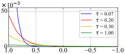
As shown in the figure, the smaller the temperature $\tau$, the larger the relative penalty for high similarity, and the larger the temperature, the more uniform the distribution of penalties.

In other words, the smaller the temperature $\tau$, the more the negative samples with high similarity of representation ($s_{i,k}(k \neq i)$) are emphasized (strongly affect the loss function) compared to the other negative samples.

For example, consider the two special cases for temperature $\tau$ ($\tau \rightarrow 0^+, \tau \rightarrow +\infty$).

First, for $\tau \rightarrow 0^+$, the loss function can be approximated as follows.

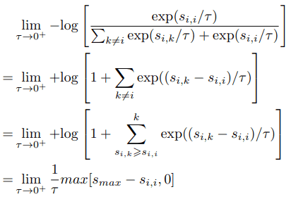
As the equation shows, in the extreme case where $\tau$ is as close to zero as possible, only the most similar negative samples affect the loss function.

Also, for $\tau \rightarrow +\infty$, we have the following

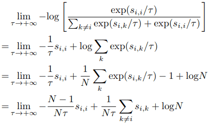
As shown in the equation, in the extreme case where $\tau$ is infinitely large, we see that the similarity of all negative samples affects the loss function without being penalized by size.

By the way, given that the purpose of Contrastive Loss is to reduce the similarity of the representation of negative samples, when the similarity $s_{i,k}(k \neq i)$ of the representation of $x_i,x_k$ is high, these are hard samples that the model fails to identify. These are hard samples that the model fails to identify.

Contrastive Loss is a Hardness-aware Loss because it is designed to penalize these difficult samples and have a larger impact on the loss function.

This hardness-aware property is critical to the success of Contrastive Loss, and in fact, training in the two extreme cases described above ($\tau\rightarrow 0^+, $\tau\rightarrow +\infty$) will either prevent the model from learning useful information (\tau \rightarrow 0^+, \tau \rightarrow +\infty$), the model will either be unable to learn useful information or will perform much worse than it would with an appropriate $\tau$ setting. Therefore, it can be said that the temperature $\tau$ plays an important role in controlling the Hardness-aware property of Contrastive Loss.

Introduction of Hard Contrastive Loss

As mentioned earlier, the Hardness-aware property, which emphasizes difficult samples with high similarity of representations, is a very important factor for Contrastive Loss.

As a more direct realization of this property, we introduce Hard Contrastive Loss, a loss function that only considers samples where $s_{i,k}$ is greater than or equal to a constant threshold $s^{(i)}_{\alpha}$.

$L_{hard}(x_i)=-log\frac{exp(s_{i,i}/\tau)}{sum{s_{i,k}\geq s^{(i)}_{\alpha}}exp(s_{i,k}/\tau)+exp(s_{i,i}/\tau)}$

Also, the relative penalty $r_i$ in this case is as follows.

$r_i(s_{i,l})=\frac{exp(s_{i,l}/\tau)}{\sum_{s_{i,k} \geq s^{(i)}_{\alpha}}exp(s_{i,k}/\tau)}, l \neq i$

This Hard Contrastive Loss can be used to penalize difficult samples by either explicitly adding the Hardness-aware property by selecting only the top $K$ negative samples, or implicitly by using the Hardness-aware property by $\tau$ described above. to difficult samples. In the following, we will analyze the Hard Contrastive Loss in addition to the usual Contrastive Loss.

On the uniformity of the embedding distribution

Existing studies have shown that uniformity of embedding distribution is an important property in contrast learning.

Based on this, we introduce a uniformity index defined by the following equation

$L_{uniformity}(f;t)=log E_{x,y～p_{data}}[e^{-t||f(x)-f(y)||^2_2}]$．

In this case, for different temperatures $\tau$, $L_{uniformity}$ for the model trained with normal Contrastive Loss is as follows.

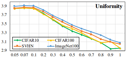
It can be seen that the larger the temperature $\tau$ is, the less uniform the embedding distribution becomes. On the other hand, the case of Hard Contrastive Loss is as follows.

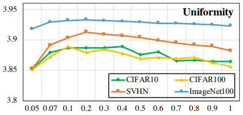
In this case, the distribution is uniform as a whole regardless of the temperature (note the value of the vertical axis), indicating that the uniformity is generally improved.

Tolerance to similar samples

Next, we analyze the acceptability of similar samples.

In contrast learning, samples generated by transforming the same image are set as positive to each other, and samples from different images are set as negative to each other, which creates the risk that the representations of samples that are actually similar (and potentially positive) are separated.

To quantitatively evaluate the tolerance to this problem (the ability not to separate the representation between similar negative samples), we measure the tolerance to similar samples based on the average similarity of samples belonging to the same class.

$T=E_{x,y~p_{data}}[(f(x)^Tf(y)) \cdot I_{l(x)=l(y)}]$

Here, $I_{l(x)=l(y)}$ is 1 when $l(x)=l(y)$ and 0 when $l(x) \neq l(y)$. The normal and Hard Contrastive Loss results for this measure are as follows.

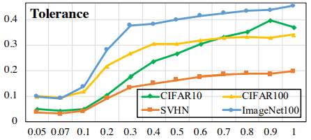
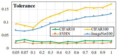
The upper figure shows the normal result and the lower figure shows the Hard Contrastive Loss result. The Hard Contrastive Loss shows a decrease in the overall index value (note the value on the vertical axis), but the change with temperature is suppressed.

However, the decrease in this index is also associated with an increase in uniformity (i.e., a decrease in the similarity of samples belonging to different classes), and it may be possible to increase the acceptability of similar samples while reducing the decrease in uniformity, especially if the temperature is relatively high.

Normal Contrastive Loss has a trade-off with Uniformity-Tolerance (we call this the Uniformity-Tolerance dilemma ). Hard Contrastive Loss deals with this problem to some extent, since it suffers from the defect that similar samples are separated as negative samples.

experimental results

In our experiments, we perform various evaluations on pre-trained models using CIFAR10, CIFAR100, SVHN, and ImageNet100 (see the original paper for the specific experimental setup).

On the effect of temperature $\tau$.

We will actually evaluate the effect of temperature on Contrastive Loss.

Specifically, we calculate $s_{i,j}$ for some anchor sample $x_i$ and all samples $x_j$, and observe the distribution of positive similarity $s_{i,i}$, top 10 negative samples $s_{i,l} \in Top_{10}(\{s_{i,j}|\forall j \neq i\})$. for the distribution of The result is as follows.

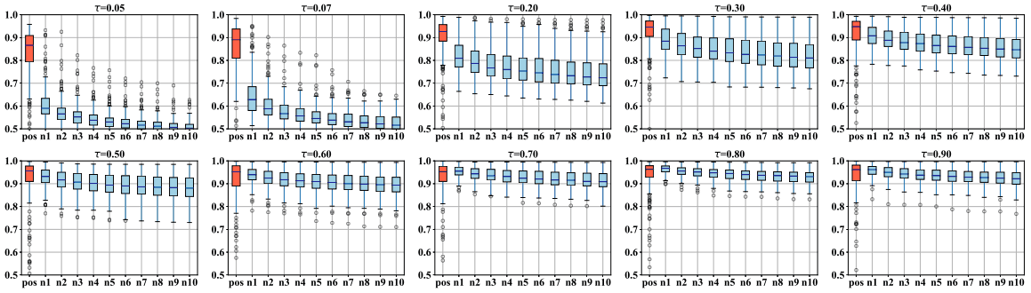
As shown in the figure, the smaller the temperature $\tau$ is, the larger the difference between positive and negative samples becomes, and the larger $\tau$ is, the closer the positive similarity is to 1 and the smaller the difference between positive and negative samples becomes. The normal and Hard Contrastive Loss results for the case where the linear layer is added after pre-training and only the linear layer is trained for 100 epochs are as follows.

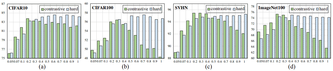
In general, the performance of Hard Contrastive Loss is good at high temperatures, while the performance at the normal (contrastive) setting tends to be in an inverted U-shape with respect to temperature. This is due to the fact that Hard Contrastive Loss guarantees uniformity at high temperatures.

When replaced by a simple loss

To confirm the claim that the Hardness-aware property is important in Contrastive Loss to properly penalize difficult negative samples, we replace the loss function with a simpler form. First, as an example without the Hardness-aware property, we introduce the following simple loss function.

$L_{simple}(x_i)=-s_{i,i}+\lambda \sum_{i \neq j}s_{i,j}$

For this simple example (Simple), when only the 4095 features with the highest similarity are used as negative samples (HardSimple), the performance on each data set is as follows.

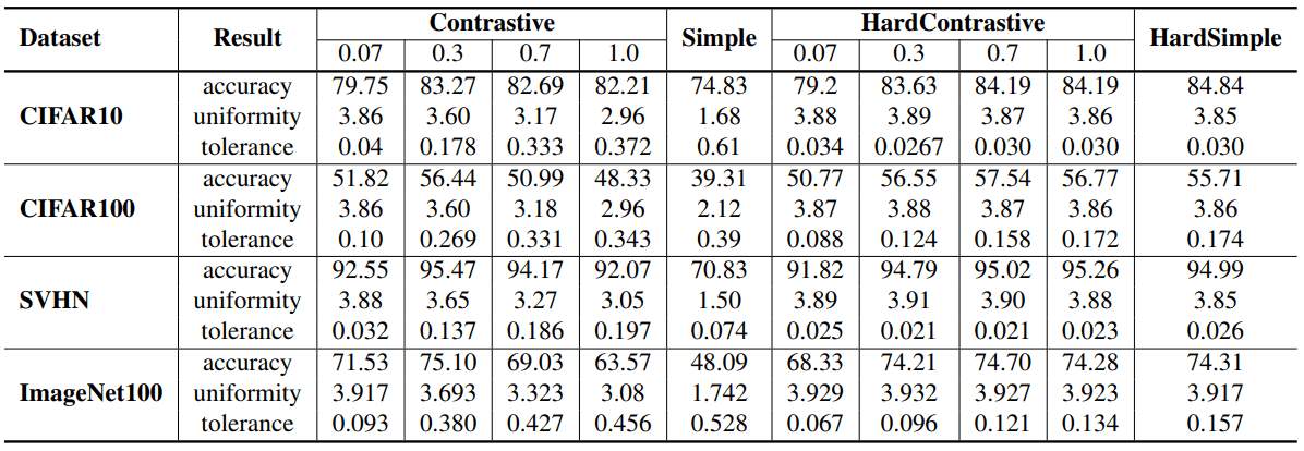
As shown in the table, the performance of the Simple setting without the Hardness-aware property is significantly worse than that of the normal and Hard Contrastive Loss, while the HardSimple setting with the Hardness-aware property shows comparable results (despite the simplicity of the loss function). in spite of the simplicity of the loss function. This shows that the hardness-aware property is important for the success of Contrastive Loss.

summary

In this article, we have presented a paper that addresses the understanding of the behavior of Contrastive Loss used in contrast learning. In general, it was shown that the Hardness-aware property is important for the success of Contrastive Loss.

We also address the dilemma of uniformity of embedding distributions and tolerance to similar samples due to the nature of contrast learning, which keeps embedding between similar negative samples away.

It is hoped that analysis of contrastive learning will continue to progress and new insights will be gained.

Categories related to this article