The Age Of Inverse Reinforcement Learning On YouTube? What Do Robots Need To Learn From Humans?
3 main points
✔️ Study on imitation learning under different hardware of learning agent and teacher agent
✔️ By capturing correspondence between videos of different teacher agents' demonstrations using self-supervised learning, we learn a reward function based on "degree of task progress", a concept that is independent of hardware differences.
✔️ We constructed X-MAJICAL as a validation dataset for a human-to-robot transition task and showed that it can learn a valid reward function even when the learning agent's equipment is unknown.
XIRL: Cross-embodiment Inverse Reinforcement Learning
written by Kevin Zakka, Andy Zeng, Pete Florence, Jonathan Tompson, Jeannette Bohg, Debidatta Dwibedi
(Submitted on Mon, 7 Jun 2021)
Comments: CoRL2021
Subjects: Robotics (cs.RO); Artificial Intelligence (cs.AI); Computer Vision and Pattern Recognition (cs.CV); Machine Learning (cs.LG)
code:
The images used in this article are from the paper, the introductory slides, or were created based on them. Mathematical formulas not shown in the paper (or not numbered in the paper) are numbered in the Roman alphabet. Mathematical formulas that are numbered in the paper are quoted as they are in the paper.
first of all
Imitation learning (IL) is a method that collects behavioral data from a teacher agent and uses statistical methods to acquire a learning agent that mimics the behavior of the teacher agent. Among them, Behavior Cloning Inverse reinforcement learning (IRL) expresses the "intention" of the teacher agent from the behavioral data of the desired task Reward function and then, using the estimated reward function Reinforcement learning (RL) and imitate the teacher agent by using the estimated reward function. Policy learning method. This framework can learn strategies in unknown environments as long as the reward function can be evaluated, so it is more efficient than supervised learning methods such as Behavior Cloning (BC) and other supervised learning methods. Therefore, inverse reinforcement learning is known as a suitable learning method for tasks that require sequential decision-making in unknown situations, such as robot control and medical diagnosis.
Usually, in inverse reinforcement learning, we assume the hardware identity of the teacher agent and the learning agent. For example, when learning a robot that performs the task of "pouring water into a glass we need to teleoperate a robot that has the same hardware as the learning agent, and repeatedly perform the task of "pouring water into a glass", and record the information of the coordinates of each joint of the robot. On the other hand, if the hardware specification of the learning agent is changed, the data collection needs to be done again, which increases the cost of data collection in the trial-and-error phase at the beginning of the project. In the early trial-and-error phase of the project, the cost of data collection increases.
In recent years, we do not require the hardware identity of the teacher agent and the learning agent Third-person imitation learning The following is the focus of this paper. In this framework, human behavior data are used as teacher data when learning a robot to perform the desired task, thus avoiding the rework of data collection that occurs every time the hardware specification of the learning agent is changed. On the one hand, human behavior data is used as the teacher data for learning robots to perform tasks. On the other hand, Since there is a hardware difference (embodiment gap) between the teacher agent and the learning agent, it is necessary to acquire the correspondence between the actions of the teacher agent and the learning agent by some means.
Challenge 1: Not only are videos shot in different environments, from different angles of view, but experts use different tools and strategies to perform the same task with different objectives.
Issue 2. : There is an EMBODYMENT GAP between humans and robots. For example, in the task of "putting five pens in a cup", a human can scoop up five pens at once using his/her hand, but a two-finger gripper robot pens one by one. In both cases, the goal can be achieved, but it is very difficult to label the correspondence between the human and the robot's actions. This problem becomes even more serious when various environments and human demonstration videos are used as training data.
The approach of this study: In this research, we learn a reward function based on "task progress", which is an invariant concept about the action subject. The reward function based on the "degree of progress in the task" is learned.
Proposed method: In this study, we learn a reward function that reflects the "degree of task progress", which is an invariant concept among operating entities.
Experimental: Constructed X-MAGICAL dataset; achieved SOTA performance on X-MAGICAL dataset and existing human-to-robot transfer benchmarks.

previous work
In this section, we outline prior work on Bayesian inverse reinforcement learning (Ramachandran & Amir, 2007). In the following, we assume that a set of behavioral data $\mathcal{D} = \{\tau_1, \tau_2, \cdots, \tau_N \}$ for the desired task has been obtained. Each behavioral data $\tau_n$ is represented as a series of data consisting of pairs of states $s\in\mathcal{S}$ and behaviors $a\in\mathcal{A}$.
$$ \tau = \{(s_0, a_0), (s_1, a_1), \cdots, (s_T, a_T)\} \tag{a}$$
In Bayesian inverse reinforcement learning, the state action value in state $S$. $Q^{\pi}_{R}$ is maximized in state $s$, and the optimal strategy $\pi(s)$ is the optimal strategy $\pi(s)$ is to select the action $a$ that maximizes the state action value is the optimal policy $\pi(s)$.
$$ \pi(s) \in \underset{a\in\mathcal{A}}{\operatorname{argmax}}Q^{\pi}_{R}(s, a) \tag{b}$$
where $Q^{\pi}_{R}$ is the Q function ( state-action value function), and Perform action $a$ in state $s$ in an environment with a known reward function $R$, and then follows the policy $\pi$. in the case where The expected total reward to be earned by $R$. The total expected reward for the action $R$ is
$$ Q^{\pi}_{R}(s, a) = \mathbb{E}_{\pi, \mathcal{T}} \left\lbrack \sum_{t}\gamma^{t}R(s_t, a_t)\middle| s_0=s, a_0=a, \pi \right\rbrack \tag{c}$$
where $\gamma \in\lbrack 0, 1)$ is the discount rate, a hyperparameter that expresses the extent to which future earned compensation is considered in current decisions.
In Bayesian inverse reinforcement learning, the posterior distribution of the reward function $P(R\mid\mathcal{D})$ is estimated under the action data $\mathcal{D}$. The posterior distribution can be calculated by Bayes' theorem as follows.
$$P(R\mid \mathcal{D}) = \frac{P(\mathcal{D}\mid R)P(R)}{P(\mathcal{D})} \tag{d}$$
The $P(R)$ is the prior distribution of the reward function and represents prior knowledge about the reward function by making appropriate choices. Also, $P(\mathcal{D}\mid R)$ is the likelihood function, a quantity that represents the plausibility of obtaining the observed values of the arguments from the assumed model. In Bayesian inverse reinforcement learning, it is assumed that the likelihood function can be represented by a Boltzmann distribution with the Q function as the energy function.
$$\begin{align}P(\mathcal{D}\mid R) &= \prod_{n=1}^N P(\tau_n \mid R) \\&\propto \prod_{n=1}^N \sum_{(s, a)\in\tau_n}\exp\left(\beta Q^{\pi}_{R}(s, a)\right)\end{align} \tag{e}$$
where $\beta\in\lbrack 0, 1)$ is the inverse temperature, a hyperparameter that represents how well the demonstrator chooses the optimal behavior.
In Bayesian inverse reinforcement learning, the expected value of the reward function is approximated by the sample mean from the posterior distribution, and the Q function is estimated using the reward function obtained as the sample mean. In this case, sampling from the posterior distribution is performed using MCMC, which repeatedly selects samples using a rejection condition based on the ratio of the posterior distribution of the reward function. On the other hand, as we saw in equation (e), the likelihood function depends on the Q-function in Bayesian inverse reinforcement learning, so the Q-function needs to be calculated every time the rejection condition is computed. Therefore, it is difficult to apply this method to the problem setting that deals with a large-scale state space from the viewpoint of computational complexity.
proposed method
In this paper, we propose an algorithm that does not require sampling from the posterior distribution of the reward function, which is a bottleneck of conventional Bayesian inverse reinforcement learning. In this section, we explain the derivation process of the objective function of the proposed method. First, the problem of finding the approximate posterior distribution $q_{\mid\mathcal{D})$ of the posterior distribution $P(R\mid\mathcal{D})$ can be written as a problem of minimizing the KL divergence between the distributions where $q_{{C}}$ is the KL divergence between the distributions.

(6) Equation can be expanded according to the definition of KL divergence and transformed into the following equation

where $\mathcal{F}(\phi)$ is a quantity called variational Lower BOund (Evidence Lower BOund, ELBO) and it is known that the maximization problem of the variational lower bound is equivalent to the optimization problem in equation (6). Furthermore, by replacing the likelihood function in the expectation of the first term in Eq. (7) with Eq. (e), the objective function can be written down as
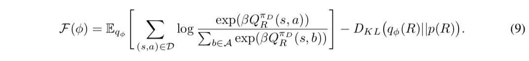
Here, since it is difficult to calculate the expectation value calculation for the approximate posterior distribution $q_{\phi}$ of equation (9) analytically, it is calculated approximately by the sample mean from $q_{\phi}$. At this time, since the likelihood function inside the expected value depends on the Q function, it is necessary to calculate the Q function for each sample of the reward function to calculate the sample average. Therefore, the iterative computation of the Q-function becomes a bottleneck, and there remains a problem from the viewpoint of computational complexity in the problem setting where a large number of states are handled. Therefore, in the proposed method, we introduce a function approximation $\mathbb{E}_{R\sim q_{\phi}}\lbrack R \rbrack$, which represents the Q function for the expected value of the reward function $\mathbb{E}_{R\sim q_{\phi}}\lbrack$ concerning the approximate posterior distribution $q_{\phi}$ is trained at the same time. In this case, the update of the Q function and the reward functionBellman equation The Bellman equation is a recursive equation of the Q-function. The Bellman equation is an expression that gives a recursive definition of the Q function and can be written down using the reward function $R$ as
$$ R(s, a) = \mathbb{E}_{\pi, \mathcal{T}}\lbrack Q(s, a) - \gamma Q(s^{\prime}, a^{\prime}) \rbrack \tag{f} $$
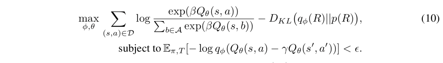
Therefore, we may add as a constraint that the negative log-likelihood of $q_{\phi}$ is less than a sufficiently small positive number $\epsilon$ in the value of the reward function calculated using the function approximator $Q_{\theta}$ that represents the Q function.
$$ - \log q_{\phi}\left( \mathbb{E}_{\pi, \mathcal{T}}\lbrack Q(s, a) - \gamma Q(s^{\prime}, a^{\prime}) \rbrack\right) < \epsilon \tag{g} $$
Based on the above, we can obtain the optimization problem of equation (10) as an approximation of the optimization problem of equation (9). (The following equation (10) is quoted as it is from the paper, but it seems that there is a typographical error in the notation of the constraint condition. The constraint condition is supposed to be correctly expressed by equation (g)).
Furthermore, by rewriting the objective function in equation (10) using the Lagrange undetermined multiplier method and approximating the expectation of the constraints by the sample mean of the behavioral data, we obtain the objective function $\mathcal{F}(\phi, \theta, \mathcal{D})$.
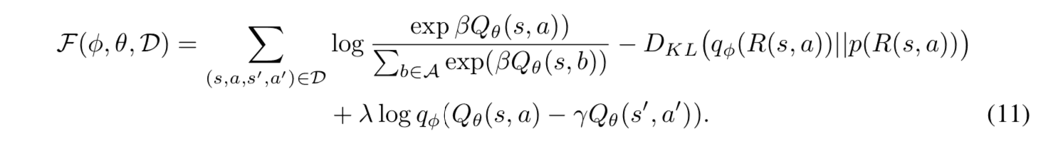
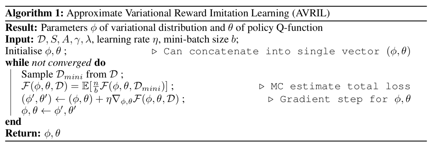
where $\lambda$ is a positive constant that determines the strength of the influence of the constraints. The proposed method iteratively updates the model based on the gradients concerning $\theta$ and $\phi$ in equation (10). The pseudo code of the learning algorithm is shown below.
experiment
In this study, we propose a Grid World task, a control task on a continuous state space, and an online medical diagnosis task. the superiority of the proposed method is shown The following section describes the contents and results of each experiment. This section describes the contents and results of each experiment.
Grid World
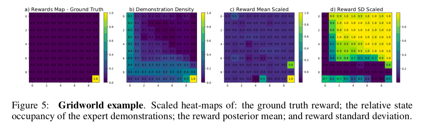
The goal of this task is to reach the target point by transitioning between states arranged on a board. In the figure below, a) is the true reward function designed manually, b) is the frequency distribution of the teacher data visiting each state, c) is the sample mean of the learned reward function, and d) is the standard deviation of the samples visualized in a heatmap. It can be said that a) and c) are close to the true reward function. Comparing b) and d), we can see that the standard deviation of samples from the posterior distribution is larger in the region with low visit frequency in the teacher data (the upper right region in the figure), indicating that the estimation uncertainty of the reward function is high. Thus, Bayesian inverse reinforcement learning has the advantage that the "reliability" of the estimation of the reward function can be quantified, and the safety of the strategy can be evaluated.
Control Tasks on Continuous State Space
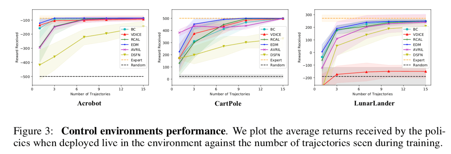
In this experiment, three different robot control tasks (Acrobat, CartPole, and LunarLander) on OpenAI gym are compared with the benchmark method sample complexity with the benchmark methods on three different robot control tasks (Acrobat, CartPole, and LunarLander). The sample complexity is roughly defined as the amount of teacher data required for the model to reach a sufficient inference performance, and the lower the sample complexity, the less teacher data is required to train the model. The figure below shows a plot of the number of teacher data on the horizontal axis and the total reward on the vertical axis for each control task. From this figure, we can see that the proposed method (AVRIL, Pink) achieves the same performance as the experts in all tasks with the same number of teacher data as the other benchmark methods. Since the other benchmark methods are based on the point estimation of the reward function, it can be said that the proposed method can learn more informative results (posterior distribution of the reward function) with the same amount of teacher data.
Offline Medical Diagnostic Tasks
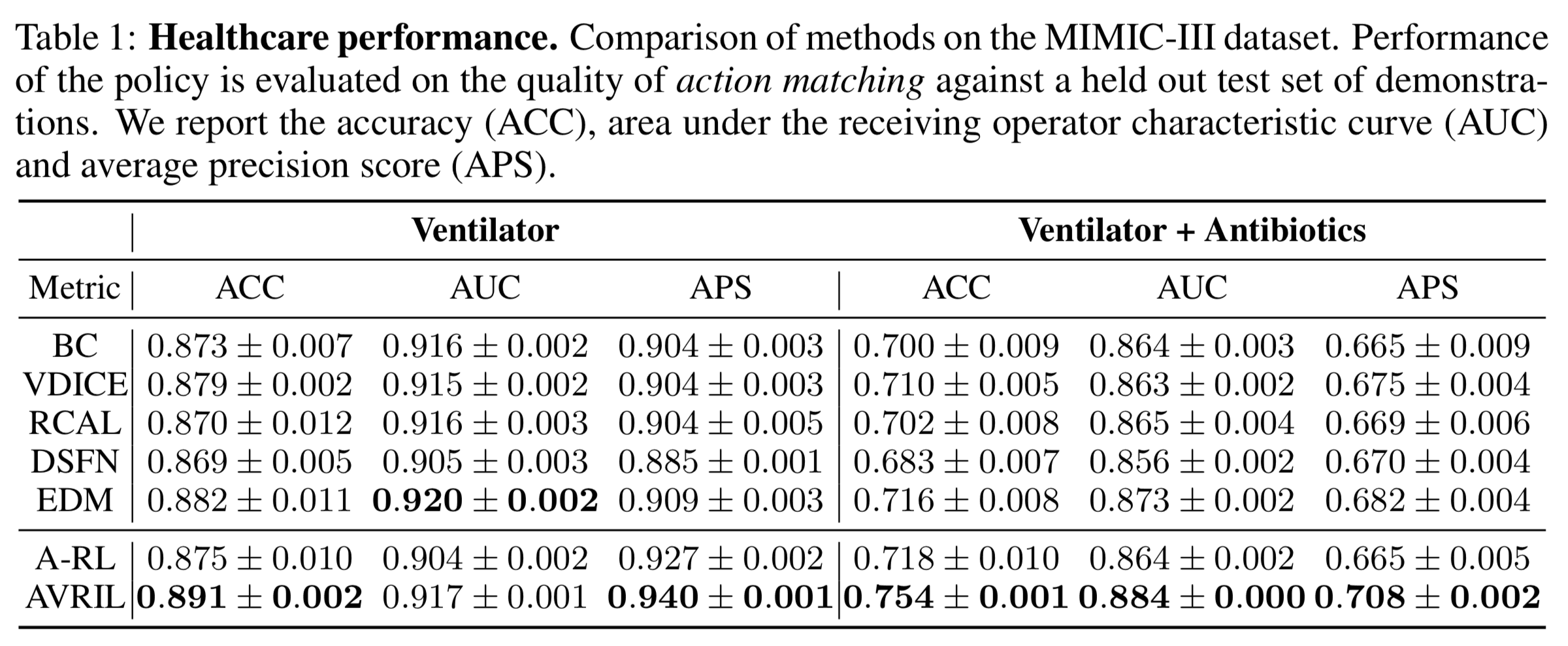
In recent years, learning strategies that enable appropriate decision-making in tasks where environment exploration is costly, such as physical robot control, or where environment exploration is ethically problematic, such as medical diagnosis, has attracted attention. Offline reinforcement learning has been the focus of much attention. In this experiment, we evaluate the performance of MIMIC-III on a decision-making task related to medical diagnosis using the MIMIC-III dataset, in which the patient's condition in the intensive care unit and the doctor's intervention are recorded every other day. Three metrics are used for evaluation: ACC (ACCuracy), AUC (Area Under the receiving operator Characteristic curve), and APC (Average Precision Score). The left side of the figure below shows the evaluation result of "whether or not the patient should be put on a ventilator", and the right side shows the evaluation result of "whether or not the patient should be given antibiotic therapy" in addition to that. It can be seen that the proposed method (AVRIL) generally outperforms the benchmark methods in both tasks. The A-RL is a model that learns a Q-function for the sample mean from the posterior distribution of the reward function learned by the proposed method, but the measures based on the Q-function acquired in the AVRIL learning process show better inference performance.
summary
In this paper, we described scalable Bayesian inverse reinforcement learning. Since Bayesian inverse reinforcement learning learns the posterior distribution of the reward function, it is possible to estimate the uncertainty of the inference result of the reward function. However, conventional methods are difficult to apply to problems with a large number of states, such as robot control tasks, from the viewpoint of computational complexity. The algorithm introduced in this paper is scalable to problems with a large number of states by avoiding MCMC iterations, which is the bottleneck of conventional Bayesian inverse reinforcement learning. Using this framework, we can learn measures to achieve the goal while avoiding the states where the estimation accuracy of the reward function is low and may be able to achieve safe imitation learning in practical tasks in the real world. Why don't you give it a try?


Categories related to this article
