Featuring Offline Reinforcement Learning! Part 2
3 main points
✔️ Off-line Evaluation with Imporatance Sampling
✔️ Off-line RL with Dynamic Programming
✔️ Mitigating Distributional Shifts through Policy Constraints and Uncertainty Estimation
Offline Reinforcement Learning: Tutorial, Review, and Perspectives on Open Problems
written by Sergey Levine, Aviral Kumar, George Tucker, Justin Fu
(Submitted on 4 May 2020)
Comments:
Subjects: Machine Learning (cs.LG), Artificial Intelligence (cs.AI), Machine Learning (stat.ML)
Introduction
In the first part of the Offline RL special edition, We introduced the overview, the applications and the problems of Offline RL. This article is a continuation of the previous one, explaining in detail the methods of Offline RL, especially the ones related to off-policy RL. If you haven't read the first part yet, please take a look at the first part first, as it will help you understand the flow of the article better.
In this article, we introduce two main methods: one is to estimate the policy return and policy gradient by using importance sampling and the other is to use dynamic programming.
Offline Evaluation and RL with Importance Sampling
First, we will investigate offline RL, which is based on a method for directly estimating policy returns and other factors. The methods we will discuss in this chapter use Impace Sampling to evaluate the returns on a given policy, or to estimate the policy gradient of the returns. The most direct method is the estimation of $J(\pi)$(objective function) in the trajectory obtained from $\pi_{\beta}$ by using importance sampling, which is called off-policy evaluation. In the next section, I will show how this off-policy evaluation is expressed in the formula and how it can be used in offline RL.
Off-policy Evaluation by Importance Sampling
You can use importance sampling to obtain an unbiased estimator of $J(\pi)$ on the off-policy trajectory.
$$\begin{aligned} J\left(\pi_{\theta}\right) &=\mathbb{E}_{\tau \sim \pi_{\beta}(\tau)}\left[\frac{\pi_{\theta}(\tau)}{\pi_{\beta}(\tau)} \sum_{t=0}^{H} \gamma^{t} r(\mathbf{s}, \mathbf{a})\right] \\ &=\mathbb{E}_{\tau \sim \pi_{\beta}(\tau)}\left[\left(\prod_{t=0}^{H} \frac{\pi_{\theta}\left(\mathbf{a}_{t} \mid \mathbf{s}_{t}\right)}{\pi_{\beta}\left(\mathbf{a}_{t} \mid \mathbf{s}_{t}\right)}\right) \sum_{t=0}^{H} \gamma^{t} r(\mathbf{s}, \mathbf{a})\right] \approx \sum_{i=1}^{n} w_{H}^{i} \sum_{t=0}^{H} \gamma^{t} r_{t}^{i} \end{aligned}$$
In the above formula, $w_{t}^{i}=\frac{1}{n} \prod_{t^{\prime}=0}^{t} \frac{\pi_{\theta}\left(\mathbf{a}_{t^{\prime}}^{i} \mid \mathbf{s}_{t^{\prime}}^{\mathrm{i}}\right)}{\pi_{\beta}\left(\mathbf{a}_{t^{\prime}}^{i} \mid \mathbf{s}_{t^{\prime}}^{i}\right)}$, and $\left\{\left(\mathbf{s}_{0}^{i}, \mathbf{a}_{0}^{i}, r_{0}^{i}, \mathbf{s}_{1}^{i}, \ldots\right)\right\}_{i=1}^{n}$ shows the trajectory sampled from n $\pi_{\beta}$. There is a problem with this estimator. However, the estimator has a problem with a large variance as it multiplies the importance weight $w$ by the horizon $H$. To solve this problem, taking advantage of the fact that $r_{t}$ does not depend on $s_{t'}$ and $a_{t'}$ at future time $t'$, we can erase the future importance weight, which can be expressed as follows
$$J\left(\pi_{\theta}\right)=\mathbb{E}_{\tau \sim \pi_{\beta}(\tau)}\left[\sum_{t=0}^{H}\left(\prod_{t^{\prime}=0}^{t} \frac{\pi_{\theta}\left(\mathbf{a}_{t} \mid \mathbf{s}_{t}\right)}{\pi_{\beta}\left(\mathbf{a}_{t} \mid \mathbf{s}_{t}\right)}\right) \gamma^{t} r(\mathbf{s}, \mathbf{a})\right] \approx \frac{1}{n} \sum_{i=1}^{n} \sum_{t=0}^{H} w_{t}^{i} \gamma^{t} r_{t}^{i}$$
This eliminates the need to multiply future importance weights, which makes the variance lower than the original formula. However, even with such a device, the variance is still generally considered to be high. The only goal is to obtain a high probability guarantee for the performance of the policy, and this importance sampling has been used in studies to obtain confidence intervals. In particular, for applications where the safety of Offline RL is important, it is necessary to improve the behavioral policy $\pi_{\beta}$ with the guarantee that the performance of the policy will not be lower than a certain level (e.g., no accidents). The first step is to use the To ensure that this safety constraint is met, research has been done to explore policies using the lower confidence bounds of the importance sampling estimator.
Off-Policy Policy Gradient
As explained at the beginning of this chapter, it is possible to directly estimate the policy gradient using import sampling, which is a way to estimate the gradient for the desired policy parameters in order to optimize $J(\pi)$. This gradient can be estimated using the Monte Carlo sample, but it requires an on-policy trajectory ($\tau \sim \pi_{\theta}$). So how can this be extended to offline RL?
Previous studies have shown that the off-policy setting, i.e., the behavior policy $\pi_{\beta}(a|s)$ and $\pi(a|s)$ are different from the off-line, but unlike the off-line, the off-policy policy gradient has collected in the past As well as reusing the data, we get new samples from behavior policy as we learn it. In this section, we introduce the off-policy gradient and show what problems and challenges we face in extending it to offline later.
The policy gradient is expressed as
$$\nabla_{\theta} J\left(\pi_{\theta}\right)=\sum_{t=0}^{H} \mathbb{E}_{\mathbf{s}_{t} \sim d_{t}^{\pi}\left(\mathbf{s}_{t}\right), \mathbf{a}_{t} \sim \pi_{\theta}\left(\mathbf{a}_{t} \mid \mathbf{s}_{t}\right)}\left[\gamma^{t} \nabla_{\theta} \log \pi_{\theta}\left(\mathbf{a}_{t} \mid \mathbf{s}_{t}\right) \hat{A}\left(\mathbf{s}_{t}, \mathbf{a}_{t}\right)\right]$$
If we estimate this using importance sampling
$$\begin{aligned} \nabla_{\theta} J\left(\pi_{\theta}\right) &=\mathbb{E}_{\tau \sim \pi_{\beta}(\tau)}\left[\frac{\pi_{\theta}(\tau)}{\pi_{\beta}(\tau)} \sum_{t=0}^{H} \gamma^{t} \nabla_{\theta} \log \pi_{\theta}\left(\mathbf{a}_{t} \mid \mathbf{s}_{t}\right) \hat{A}\left(\mathbf{s}_{t}, \mathbf{a}_{t}\right)\right] \\ &=\mathbb{E}_{\tau \sim \pi_{\beta}(\tau)}\left[\left(\prod_{t=0}^{H} \frac{\pi_{\theta}\left(\mathbf{a}_{t} \mid \mathbf{s}_{t}\right)}{\beta\left(\mathbf{a}_{t} \mid \mathbf{s}_{t}\right)}\right) \sum_{t=0}^{H} \gamma^{t} \nabla_{\theta} \log \pi_{\theta}\left(\mathbf{a}_{t} \mid \mathbf{s}_{t}\right) \hat{A}\left(\mathbf{s}_{t}, \mathbf{a}_{t}\right)\right] \\ & \approx \sum_{i=1}^{n} w_{H}^{i} \sum_{t=0}^{H} \gamma^{t} \nabla_{\theta} \log \pi_{\theta}\left(\mathbf{a}_{t}^{i} \mid \mathbf{s}_{t}^{i}\right) \hat{A}\left(\mathbf{s}_{t}^{i}, \mathbf{a}_{t}^{i}\right) \end{aligned}$$
When we estimate the policy gradient, we can exclude future importance weights in the same way as we did for the returns introduced in the previous section.
$$\nabla_{\theta} J\left(\pi_{\theta}\right) \approx \sum_{i=1}^{n} \sum_{t=0}^{H} w_{t}^{i} \gamma^{t}\left(\sum_{t^{\prime}=t}^{H} \gamma^{t^{\prime}-t} \frac{w_{t^{\prime}}^{i}}{w_{t}^{i}} r_{t^{\prime}}-b\left(\mathbf{s}_{t}^{i}\right)\right) \nabla_{\theta} \log \pi_{\theta}\left(\mathbf{a}_{t}^{i} \mid \mathbf{s}_{t}^{i}\right)$$
Approximate Off-Policy Policy Gradient
In the import-weighted policy objective described in the previous section, we also have to multiply the import weight, which results in a large variance. So, instead of the state distribution $d^{\pi}$ in the current policy $\pi$, we can use the state distribution of $\pi_{\beta}$ to obtain the approximate policy gradient of $\pi$. This approximate policy gradient is also biased due to the mismatch between the state distribution $d^{\pi}$ and $d^{\pi_{\beta}}$, but research has shown that it often works in practice. This new objective function can be expressed as follows
$$J_{\beta}\left(\pi_{\theta}\right)=\mathbb{E}_{\mathbf{s} \sim d^{\pi} \beta(\mathbf{s})}\left[V^{\pi}(\mathbf{s})\right]$$
The $J_{\beta}(\pi_{\theta})$ and $J(\pi_{\theta})$ are in different state distributions and $J_{\beta}(\pi_{\theta})$ is a biased estimator of $J(\pi_{\theta})$. Because of the biased estimator, a suboptimal solution is sometimes required, but in the case of the objective function in $d^{\pi_{\beta}}$, there is no need to use import sampling, so we can use the The advantage is that the data can be sampled and easily calculated.
Future Challenges
In this chapter, we introduced a method of using import sampling to estimate the final return, or slope of return, on the current policy $\pi_{\theta}$ using import sampling. However, the policy improvement introduced above is basically for off-policy learning, i.e., it is designed to use both samples collected in the past and new samples collected at the same time as the training. This is why offline RL is not very useful for this purpose. So what are the problems that need to be solved in order to use offline RL? For one thing, if the behavior policy $\pi_{\beta}$ used to collect offline data is too far away from the current policy $\pi_{\theta}$, due to the high variance of the import sampling itself, then this leads to poor estimation by importance sampling and too much variance, especially in high-dimensional state and action spaces or long-horizon problems. Therefore, must not be too far from the $\pi_{\beta}$. Therefore, The condition that $\pi_{\theta}$ is not too far apart with respect to $\pi_{\beta}$ is essential. Therefore, the method using importance sampling is currently limited to low-dimensional state/action spaces or relatively short horizon tasks that use suboptimal $\pi_{\beta}$.
Off-line RL with Dynamic Programming
Algorithms using Dynamic Programming, such as Q-learnng, are basically better for Offline RL than those using policy gradient. In the case of actor-critic, the policy gradient is estimated by using the value function. There have been several studies on offline RL using dynamic programming, such as QT-Opt, which is a Q-learning method based on 500,000 offline grasping data. However, this method has also been shown to be more accurate when additional data is used at the same time as new training. However, some studies have shown that some datasets can be trained better with offline RL.
However, we know that if online data collection is not done, the distribution shift does not produce good results, as introduced in the first offline RL feature. There are two main ways to solve this problem, one is called policy constrant, which is to make the policy $\pi$ learned close to the policy $\pi_{\beta}$ used to collect the data. The other method, called uncertainty-based method, estimates the uncertainty of Q-values and uses it to discover distribution shifts. In this section, we will first explain the distribution shift in detail, introduce these two methods, and then explain what kind of problems need to be solved in the end.
Distribution Shift
There are two types of distribution shifts that can cause problems in Offline RL: state distribution shift (visitation frequency) and action distribution shift. In the state distribution shift, if the state visitation frequency dps for the learned policy p is different from the state visitation frequency dpbs of behavior policy pb when the policy p learned in offline RL is evaluated at test time, the policy trained by the actor-critic may produce unexpected actions in the unknown state. This distribution shift regarding state is a problem in testing, but the opposite is true in training, where the distribution shift regarding action is a problem. This is because $Q(s_{t+1}, a_{t+1})$ needs to be calculated in order to calculate the following target Q-value, which relies on $a_{t+1} \sim \pi(a_{t+1}|s_{t+1})$, so that if $\pi(a|s)$ is far away from $\pi_{\beta}$, you will get a target Q-value with a large error.
$$\left.Q^{\pi}\left(\mathbf{s}_{t}, \mathbf{a}_{t}\right)=r\left(\mathbf{s}_{t}, \mathbf{a}_{t}\right)+\gamma \mathbb{E}_{\mathbf{s}_{t+1} \sim T\left(\mathbf{s}_{t+1} \mid \mathbf{s}_{t}, \mathbf{a}_{t}\right), \mathbf{a}_{t+1} \sim \pi\left(\mathbf{a}_{t+1} \mid \mathbf{s}_{t+1}\right)}\left[Q^{\pi}\left(\mathbf{s}_{t+1}, \mathbf{a}_{t+1}\right)\right)\right]$$
And if the policy is able to output an unknown action, for example under a situation where the Q-functions are very large due to errors, then the policy will learn to execute the action. In online RL, the Q-function can be corrected by getting new data even if it falls into this kind of situation, but this is not possible in offline RL, so this is a problem.
It's not a matter of just adding more data. In the figure below, the horizontal axis is the gradient update, the vertical axis is the final average return on the left, and the Q-value on the log scale is on the right. If you look at the green line on the left in the diagram below, it looks like overfitting because once the performance goes up, it goes down as we continue to learn, but this is not the case when you compare it to the lesser data in the orange, where overfitting is solved by adding more data. This makes the problem more complicated. In addition, as the training progresses, the target Q-value becomes larger and the overall Q-function becomes worse. In this way, it can be said that the distribution error on action is important for learning agent effectively using offliine RL. Next, we introduce the policy constraint as one of the solutions to this problem.
Policy Constraints
One effective way to prevent a distribution shift on an action is to use a policy constraint to keep $\pi(a|s)$ close to $\pi_{\beta}(a|s)$ and prevent an unknown action from being executed. If an unknown action is executed, errors will continue to accumulate as a result of the unexpected action being executed once, but if the unknown action is not executed, the accumulation of errors will be prevented. So how do we do policy constrant? In this article, we discuss explicit f-divergene constraints, implicit f-divergence constraints (mainly KL-divergence), and a technique called the integral probability metric (IPM) We will introduce them. There are also two basic types of constraints: policy constraints, which directly constrain the actors' updates, and policy penalties, which constrain the reward function and target Q-value.
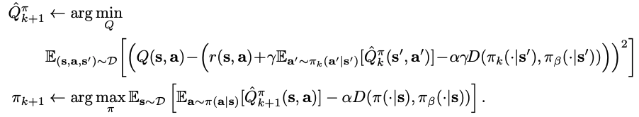
First, let's look at policy constraints, which can be expressed as a fixed point iteration method with the following objectives
$$\hat{Q}_{k+1}^{\pi} \leftarrow \arg \min _{Q} \mathbb{E}_{\left(\mathbf{s}, \mathbf{a}, \mathbf{s}^{\prime}\right) \sim \mathcal{D}}\left[\left(Q(\mathbf{s}, \mathbf{a})-\left(r(\mathbf{s}, \mathbf{a})+\gamma \mathbb{E}_{\mathbf{a}^{\prime} \sim \pi_{k}\left(\mathbf{a}^{\prime} \mid \mathbf{s}^{\prime}\right)}\left[\hat{Q}_{k}^{\pi}\left(\mathbf{s}^{\prime}, \mathbf{a}^{\prime}\right)\right]\right)\right)^{2}\right]$$
$$\pi_{k+1} \leftarrow \arg \max _{\pi} \mathbb{E}_{\mathbf{s} \sim \mathcal{D}}\left[\mathbb{E}_{\mathbf{a} \sim \pi(\mathbf{a} \mid \mathbf{s})}\left[\hat{Q}_{k+1}^{\pi}(\mathbf{s}, \mathbf{a})\right]\right]$ s.t. $D\left(\pi, \pi_{\beta}\right) \leq \epsilon$$
This is basically the general actor-critic method with the addition of the constraint $D\left(\pi, \pi_{\beta}\right) \leq \epsilon$ to the general actor-critic method. The $D$ has been experimented with in the past, including some studies with different choices. This is called a policy constraint that adds a constraint on the actors' update.
Now let's look at the policy penalty. In the Actor-critic, a constraint is added to the Q-value to ensure that the policy $\pi$ is not too far from $\pi_{\beta}$, and prevent them from choosing actions that would take them away from $\pi_{\beta}$ in the future. This can be done by adding a penalty $\alpha \mathcal{D}(\pi(\cdot|s), \pi_{\beta}(\cdot|s))$ to the reward function, i.e., $\bar{r}(\mathbf{s}, \mathbf{a})=r(\mathbf{s}, \mathbf{a})-\alpha D\left(\pi(\cdot \mid \mathbf{s}), \pi_{\beta}(\cdot \mid \mathbf{s})\right)$. Another method of adding constraint$\alpha D\left(\pi(\cdot \mid \mathbf{s}), \pi_{\beta}(\cdot \mid \mathbf{s})\right)$ directly to the target Q-value has been proposed and can be expressed as
Now let's look at the different types of constraints. The first one is the explicit f-divergence constraints. For all $f$ convex functions $f$, $f$-divergence is defined as follows.
$$D_{f}\left(\pi(\cdot \mid \mathbf{s}), \pi_{\beta}(\cdot \mid \mathbf{s})\right)=\mathbb{E}_{\mathbf{a} \sim \pi(\cdot \mid \mathbf{s})}\left[f\left(\frac{\pi(\mathbf{a} \mid \mathbf{s})}{\pi_{\beta}(\mathbf{a} \mid \mathbf{s})}\right)\right]$$
KL-divergence, $\chi^{2}$ -divergence, and total-variance distance are some of the most commonly used types of $f$-divergence.Next, we introduce implicit f-divergence constraints.
Implicit $f$-divergence constraints are AWR andABM and other models, and we will train the policy in the following steps.
$$\begin{aligned} \bar{\pi}_{k+1}(\mathbf{a} \mid \mathbf{s}) & \leftarrow \frac{1}{Z} \pi_{\beta}(\mathbf{a} \mid \mathbf{s}) \exp \left(\frac{1}{\alpha} Q_{k}^{\pi}(\mathbf{s}, \mathbf{a})\right) \\ \pi_{k+1} & \leftarrow \arg \min _{\pi} D_{\mathrm{KL}}\left(\bar{\pi}_{k+1}, \pi\right) \end{aligned}$$
In the first expression above, the importance sampling weight $\exp \left(\frac{1}{\alpha} Q_{k}^{\pi}(\mathbf{s}, \mathbf{a})\right)$ is weighted against the sample on $\pi_{\beta}(a|s)$, and by solving the problem of regression using KL-divergence, we determine the following policy. $\alpha$ is the Lagrangian multiplier. You can check the derivation for this method here.
Finally, we will introduce Integral probability metrics (IPMs). It is such that divergence can be measured by the following formula, where $D_{\Phi}$ depends on the function class $\Phi$.
$$D_{\Phi}\left(\pi(\cdot \mid \mathbf{s}), \pi_{\beta}(\cdot \mid \mathbf{s})\right)=\sup _{\boldsymbol{d} \in \mathbf{\Phi}}\left|\mathbb{E}_{\mathbf{a} \sim \pi(\cdot \mid \mathbf{s})}[\phi(\mathbf{s}, \mathbf{a})]-\mathbb{E}_{\mathbf{a}^{\prime} \sim \pi_{\beta}(\cdot \mid \mathbf{s})}\left[\phi\left(\mathbf{s}, \mathbf{a}^{\prime}\right)\right]\right|$$
For example, if the function class $\Phi$ is reproducing kernel Hilbert space (RKHS), then $D_{\Phi}$ represents the maximum mean discrepancy (MMD). This MMD-based method is used in a method called BEAR.
So how do I choose a constraint? Basically, KL-divergence and other $f$-divergences are not well suited for offline RL. For example, if the behavioral policy is uniformly random, KL-divergence makes the policy closer to the behavioral policy, which results in a very stochastic suboptimal policy. In contrast, some research suggests that restricting the support (platform) of a policy $\pi(a|s)$ to a platform of behavioral policy is more effective for offline RL. Let's look at the 1-D Lineworld Environment example below. In this example, we start from Start $S$ and go to Goal $G$, and the behavior policy is assumed to have a high probability of transition to the left as shown in (b). In this case, when distribution-matching (e.g., KL-divergence) is used, it is not possible to find the best policy because it matches with a behavior policy that has a high probability of transitioning to the left. On the other hand, support-constraint is said to help you find the best policy. The support constraint is made possible by the constraint using the Maximum Mean Discrepancy introduced above, and it has been shown in the past that the constraint works similarly to the constraint on distribution as well as support. Research shows this experimentally.
Uncertainty Estimation
Next, I will introduce a method of uncertainty estimation for distribution shift that is different from the policy constraint. The main idea of this method is to output a conservative target Q-value using the uncertainty about unknown actions, since the uncertainty about unknown actions increases when the uncertainty about the Q-function can be estimated. The method must learn the set or distribution of uncertainties in the Q-function represented by $\mathcal{P}_{\mathcal{D}}\left(Q^{\pi}\right)$. And if we can learn this set of uncertainties, we can improve the policy by estimating the conservative Q-function. This equation is expressed as follows, where $Unc$ represents uncertainty, and we subtract this from the estimate of the actual Q-value.
$$\pi_{k+1} \leftarrow \arg \max _{\pi} \mathbb{E}_{\mathbf{s} \sim \mathcal{D}} \underbrace{\left[\mathbb{E}_{\mathbf{a} \sim \pi(\mathbf{a} \mid \mathbf{s})}\left[\mathbb{E}_{Q_{k+1}^{\pi} \sim \mathcal{P}_{\mathcal{D}}\left(Q^{\pi}\right)}\left[Q_{k+1}^{\pi}(\mathbf{s}, \mathbf{a})\right]-\alpha \operatorname{Unc}\left(\mathcal{P}_{\mathcal{D}}\left(Q^{\pi}\right)\right)\right]\right]}_{\text {conservative estimate }}$$
The main ways to compute this $Unc$ are to do an ensemble of Q-functions or to maximize the Q-value of the worst-case.
Future Challenges
As explained in this chapter, the approximate dynamic programming algorithm performs poorly in offline settings, mainly due to distributive shifts in action, and the policy I have introduced two types of solutions: constraint and uncertainty estimation. However, although uncertainty estimation does not provide better performance than policy constraint, it is still a good idea to use uncertainty estimation when there is a need to perform actions conservatively (e.g., to prevent accidents), especially in offline RL. This use of uncertainty estimation is particularly important and needs to be improved in the future. On the other hand, policy constraint has performed somewhat better, but the performance of the algorithm using policy constraint is not as good as that of It depends on the accuracy of behavior policy estimation. In other words, if behavior policy shows multimodal behavioral movements, it is difficult to accurately estimate behavior policy, and it is currently difficult to apply behavior policy to real-world problems. In addition, even if the behavior policy is perfectly estimated, learning may not proceed due to the effects of function approximation. For example, if the dataset is small, it may overfitting a small dataset, and if the action-state distribution is very narrow, the learned policy will be generic. And above all, while online RL solves the overestimation error by collecting new data, offline RL has the problem of the error piling up. And the other problem is that once the training policy leaves the behavior policy, it gets further and further away from theThe performance degradation occurs because of the frequent visits of learned policies to unknown states. Therefore. You need to apply a strong policy constraint, but this will limit policy improvement. Therefore, one of the things we need to consider is to find a constraint that can effectively make a trade-off between the problem of error accumulation and the problem of suboptimal policies being learned.
Summary
In this article, we have introduced the methods and problems of Offline RL in Model-free RL. However, we hope that this article will give you an overall picture of the method and help you to read the paper in the future. I'd like to keep a close eye on the problems with offline RL and its performance, but I'm not sure if the action distribution shift problem can really be solved from the offline dataset alone.


Categories related to this article