![[PiCIE] Pixel-level Clustering For Unsupervised Semantic Segmentation.](https://aisholar.s3.ap-northeast-1.amazonaws.com/media/November2021/picie.png)
[PiCIE] Pixel-level Clustering For Unsupervised Semantic Segmentation.
3 main points
✔️ Propose an unsupervised semantic segmentation method based on pixel-level clustering
✔️ Use of a loss function introducing two inductive biases (Invariance and Equivariance)
✔️ Excellent performance in COCO and Cityscapes
PiCIE: Unsupervised Semantic Segmentation using Invariance and Equivariance in Clustering
written by Jang Hyun Cho, Utkarsh Mall, Kavita Bala, Bharath Hariharan
(Submitted on 30 Mar 2021)
Comments: CVPR 2021.
Subjects: Computer Vision and Pattern Recognition (cs.CV)
code:

The images used in this article are from the paper, the introductory slides, or were created based on them.
first of all
For semantic segmentation, pixel-level annotated datasets are important.
In reality, however, such a dataset is not always available because of the high cost of image annotation.
In the paper presented in this article, we propose a method for unsupervised semantic segmentation from unlabeled datasets, as shown in the figure below.
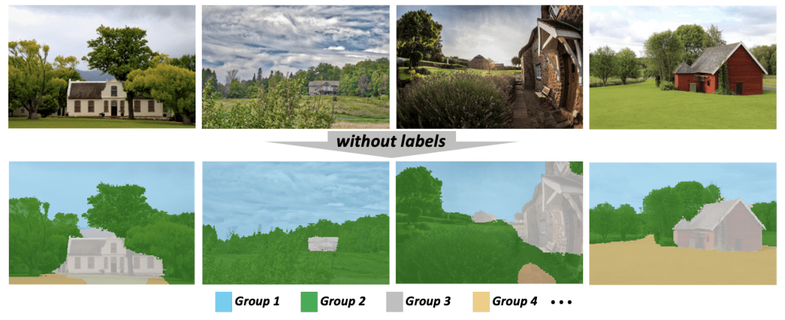
If such unsupervised semantic segmentation can be achieved, it has various advantages, such as reducing the cost of annotation and discovering classes that have not been discovered by humans.
Our proposed method, PiCIE (Pixel-level feature Clustering using Invariance and Equivariance), addresses this problem based on pixel-level clustering and outperforms existing methods. Let's take a look at it below.
The proposed method (PiCIE)
To begin, we consider the task set up for the unsupervised semantic segmentation task.
For an unlabeled image dataset from a domain $D$, the goal of this task is to discover a set of visual classes $C$ in the image and learn a function $f_{\theta}$ that assigns a class to every pixel in the image obtained from $D$.
The proposed method, PiCIE, solves this problem as pixel-level clustering, where all pixels in an image (instead of each image) are assigned to a cluster.
However, for such clustering to be done properly, each pixel must be converted into a good feature representation, but such a feature space is not given a priori.
For this reason, PiCIE performs pixel-level clustering and learns feature representations for this purpose.
Baseline with pixel-level clustering
Before considering pixel-level clustering, we address existing work on image-level clustering.
The challenge here is the dilemma that we need a good feature representation for clustering, but we need class labels to get that feature representation.
To solve this problem, DeepCluster performs clustering to find feature representations and then learns feature representations by using the clusters obtained from the clustering as pseudo-labels. This method can be extended to unsupervised semantic segmentation.
In other words, the process is to find a feature representation for each pixel, perform clustering for each pixel, and then use the pseudo-label to learn a feature representation for each pixel.
Specifically, for an unlabeled image $x_i (i=1,... ,n)$, let $f_\theta(x)$ be the feature tensor obtained by $f_\theta$, $f_\theta(x)[p]$ be the feature representation corresponding to pixel $p$, and $g_w(\cdot)$ be the classifier that classifies each pixel, the following two processes are repeated baselines can be considered.
1. clustering of each pixel of the image in the dataset using the current feature representation and k-means method (actually Mini Batch K-Means method).
$min_{y,\mu}\sum_{i,p} ||f_\theta(x_i)[p]-\mu_{y_{ip}}||^2$
where $y_{ip}$ denotes the cluster label of the $p$th pixel of the $i$th image and $\mu_k$ denotes the center point (centroid) of the $k$th cluster.
2. Based on the pseudo-labels obtained by clustering, we learn a pixel-by-pixel classifier using cross entropy loss.
$min_{\theta,w}\sum_{i,p} L_{CE}(g_w(f_\theta(x_i)[p]),y_{ip})$
$L_{CE}(g_w(f_\theta(x_i)[p]),y_{ip})=-log\frac{e^s_{y_{ip}}}{\sum_ke^{s_k}}$
where $s_k$ is the score output corresponding to the $k$th class of the classifier $g_w(f_\theta(x_i,p))$. With these as a baseline, the proposed method, PiCIE, makes the modifications described below.
Nonparametrization of classifiers
In the baseline described above, we use the classifier $g_w(\cdot)$ to classify each pixel.
However, since the pseudo-labels used to train this classifier are constantly changing during the training process, the output of this classifier may be noisy and may not work effectively.
Therefore, we do not use the pixel classifier $G_W$, but simply label pixels using the distance to the center point of each cluster.
$min_\theta \sum_{i,p}L_{clust}(f_\theta(x_i)[p],y_{ip},\mu)$
$L_{clust}(f_\theta(x_i)[p],y_{ip},\mu)=-log(\frac{e^{-d(f_\theta(x_i)[p],\mu_{y_{ip}})}}{\sum_l e^{-d(f_\theta(x_i)[p],\mu_l)}})$.
where $d(\cdot,\cdot)$ is the cosine distance.
Introduction of inductive bias
In addition to the learning procedure described above, we introduce two inductive biases for semantic segmentation.
- Invariance to photometric transformations (Iinvariance to photometric transformations): The labels are invariant even if the colors of the pixels change slightly. (For example, if the brightness of the whole image changes, the labels do not change.)
- Equivariance to geometric transformations: If the image changes geometrically, the labels will change as well. (For example, if a part of the image is enlarged, the label will be enlarged as well.)
Specifically, if the semantic label output for image $x$ is $Y$, the photometric transformation is $P$, and the geometric transformation is $G$, then the output of image $G(P(x))$ subjected to these transformations is $G(Y)$.
To ensure that the prediction results satisfy these properties, the following process is used.
On invariance to photometric transformations
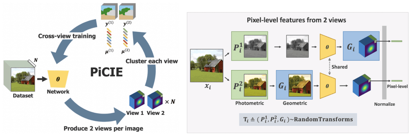
First, we consider invariance to photometric transformations.
For each image $x_i$ in the dataset, we randomly sample two photometric transformations $P^{(1)}_i$,$P^{(2)}_i$. For each image with these transforms, two feature vectors corresponding to each pixel are obtained.
$z^{(1)}_{ip}=f_\theta(P^{(1)}_i(x_i))[p]$
$z^{(2)}_{ip}=f_\theta(P^{(2)}_i(x_i))[p]$
Based on these feature vectors, we can obtain two pseudo-labels and a center point.
$y^{(1)},\mu^{(1)}=arg min_{y,\mu}_sum_{i,p}||z^{(1)}_{ip}-\mu_{y_{ip}}||2$
$y^{(2)},\mu^{(2)}=arg min_{y,\mu}_sum_{i,p}||z^{(2)}_{ip}-\mu_{y_{ip}}||2$
Based on these pseudo-labels and central points, we introduce the two loss functions shown below.
$L_{within}=\sum_{i,p}L_{clust}(z^{(1)}_{ip},y^{(1)}_{ip},\mu^{(1)})+L_{clust}(z^{(2)}_{ip},y^{(2)}_{ip},\mu^{(2)})$
$L_{cross}=\sum_{i,p}L_{clust}(z^{(1)}_{ip},y^{(2)}_{ip},\mu^{(2)})+L_{clust}(z^{(2)}_{ip},y^{(1)}_{ip},\mu^{(1)})$
By $L_{within}$, we train the feature vector clustering to work effectively (to be close to the center point corresponding to the pseudo-label) even when subjected to photometric transformation.
On the other hand, $L_{cross}$ achieves invariance to photometric transformations by learning the feature vector clustering to work effectively even for pseudo-label/center points corresponding to images undergoing different photometric transformations.
On isobaric degeneration for geometric transformations
Furthermore, we introduce an equivariant for geometric transformations. Specifically, we incorporate the geometric transformation $G_i$ into the two feature vectors described above.
$z^{(1)}_{ip} = f_\theta(Gi(P^{(1)}_i (xi)))[p]$
$z^{(2)}_{ip} = G_i(f_\theta(P^{(2)}_i (xi)))[p]$
In this case, $Z^{(1)}_{ip}$ is applied to the image $P^{(1)}_i (xi)$ undergoing the photometric transformation, and $Z^{(2)}_{ip}$ is applied to the feature vector $f_\theta(P^{(2)}_i (xi))$ of the image undergoing the photometric transformation, respectively, by the geometric transformation is performed.
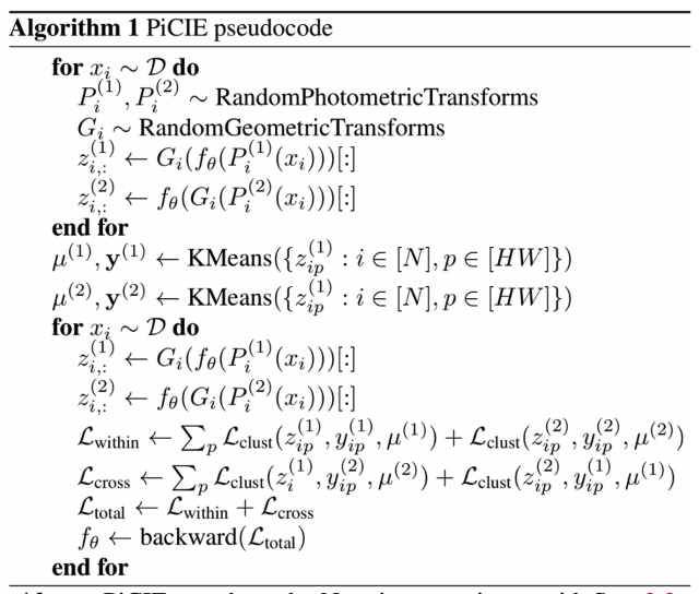
Based on these feature vectors, we can learn based on invariance and isovariance by using the loss function $L_{total}=L_{within}+L_{cross}$, which is a combination of the loss functions described earlier.
Based on these feature vectors, we learn based on invariance and isovariance by using the loss function $L_{total}=L_{within}+L_{cross}$, which combines the loss functions described earlier.
Finally, the pipeline pseudocode for PiCIE looks like this
experimental results
In our experiments, we use the COCO-Cityscapes dataset for validation (we omit the experimental setup). An example prediction of the proposed method on the COCO-Cityscapes dataset is shown below.
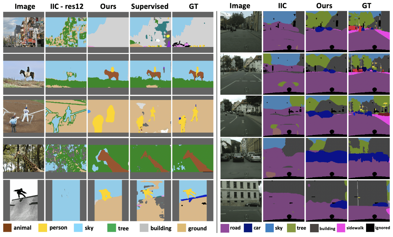
As shown in the figure, compared to the baseline existing method IIC, the proposed method shows superior prediction results. It is also comparable to Supervised and Ground Truth.
The performance on the entire COCO dataset, the performance on the two categories (Stuff/Thing), and the performance on the Cityscapes dataset are shown below, respectively.
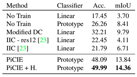
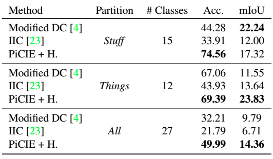

Modified DC indicates DeepCluster modified for semantic segmentation. Also, +H indicates Overclustering (joint optimization for the large number of clusters). In general, the proposed method outperforms the existing unsupervised methods.
summary
The challenging problem of unsupervised semantic segmentation was addressed in the paper presented in this article by introducing pixel-level clustering and two inductive biases and showed excellent results.
They are very simple, require no task-specific processing or fine-grained hyperparameter tuning, yet perform well on both the stuff and things categories of the COCO dataset, opening up a new avenue for unsupervised semantic segmentation. We believe that our work opens up a new avenue for unsupervised semantic segmentation.


Categories related to this article

![[Segment Anything] Z](https://aisholar.s3.ap-northeast-1.amazonaws.com/media/June2024/segment_anything-520x300.png)