Semi-supervised Segmentation With Imprecise Pseudo-labels

Segmentation 22/08/2022

3 main points
✔️ We developed a novel semi-supervised segmentation method, $U^2PL$, which uses imprecise pseudo labels for training.
✔️ Classified the pseudo labels as accurate or inaccurate by entropy and used the inaccurate labels as a cue of negative samples for each class.
✔️ In various benchmark experiments, the thesis method recorded SOTA.

Semi-Supervised Semantic Segmentation Using Unreliable Pseudo-Labels
written by Yuchao Wang, Haochen Wang, Yujun Shen, Jingjing Fei, Wei Li, Guoqiang Jin, Liwei Wu, Rui Zhao, Xinyi Le
(Submitted on 8 Mar 2022 (v1), last revised 14 Mar 2022 (this version, v2))
Comments: Accepted to CVPR 2022
Subjects: Computer Vision and Pattern Recognition (cs.CV)

code：

The images used in this article are from the paper, the introductory slides, or were created based on them.

first of all

In semi-supervised segmentation, it is important to give a sufficient number of pseudo-labels to unlabeled data. Traditional methods use pixels that are confident in their predictions as the Ground Truth but have the problem that most pixels are not confident and therefore cannot be used for training. Intuitively, a pixel with low confidence should have high confidence that it is unsure of its prediction between certain classes and does not belong to any other class. Therefore, they can be used as negative samples for those classes. In this paper, we develop a method to fully use unlabeled data. First, we classified labels by entropy value into accurate and inaccurate and used the inaccurate labels as a cue for negative samples for each class in training. As the model predictions became more accurate, we adaptively adjusted the accurate-inaccurate classification threshold.

technique

Let ${\cal D}_l=\{(x_i^l, y_i^l)\}_{i=1}^{N_l}$ for labeled data and ${\cal D}_u=\{(x_i^u)\}_{i=1}^{N_u}$. The schematic of $U^2PL$ is shown in the figure below: it consists of a Student model and a Teacher model, and the only difference between them is the way of updating the weights: the weights $\theta_s$ in the Student model are updated in the usual way, and the weights $\theta_t$ in the Teacher model are updated by $\ theta_t$ is updated by the exponential moving average of $\theta_s$. Both models consist of a CNN-based encoder $h$ and a decoder with a segmentation head $f$ and a representation head $g$. Labeled and unlabeled data ${\cal B}_l, {\cal B}_u$ of $B$ samples each were extracted at each training stage. For the labeled data, we minimized the usual cross-entropy, and for the unlabeled data, we put them in the Teacher model and minimized the pseudo cross-entropy from the entropy values to the exact labels. Finally, we used the contrastive loss to use inexact labels. The final loss function was as follows

$${\cal L}={\cal L}_s+\lambda_u{\cal L}_u+\lambda_c{\cal L}_c$$

where $\lambda_u, \lambda_c$ are balanced parameters and ${\cal L}_s, {\cal L}_u$ are labeled and unlabeled loss functions expressed as

$${\cal L}_s=\frac{1}{|{\cal B}_l|}\sum_{(x_i^l,y_i^l)\in {\cal B}_l}l_{ce}(f\circ h(x_i^l;\theta),y_i^l)$$

$${\cal L}_u=\frac{1}{|{\cal B}_u|}\sum_{x_i^u\in {\cal B}_u}l_{ce}(f\circ h(x_i^u;\theta), {\hat y}_i^u)$$

However, $y_i^l$ is the annotation label of the $i$-th labeled data, ${\hat y}_i^u$ is the pseudo label of the $i$-th unlabeled data, and $f\circ h$ is the composition function of $f$ and $h$. ${\cal L}_c$ is the following.

$${\cal L}_c=-\frac{1}{C\times M}\sum_{c=0}^{C-1}\sum_{i=1}^{M}\log\left[\frac{e^{<{\bf z}_{ci},{\bf z}_{ci}^+>/\tau}}{e^{<{\bf z}_{ci},{\bf z}_{ci}^+>/\tau}+\sum_{j=1}^Ne^{<{\bf z}_{ci},{\bf z}_{cij}^->/\tau}}\right]$$

where $M$ is the number of anchor pixels and ${\bf z}_{ci}$ is the replication of the $i$th anchor pixel of class $c$. Each anchor has $N$ positive and $N$ negative samples, and each replication is ${\bf z}_{ci}^+,{\bf z}_{cij}^-$ are. The $<\cdot,\cdot>$ is the cosine similarity and $\tau$ is the hyperparameter.

pseudo-labeling

Let ${\bf p}_{ij}\in {\mathbb R}^C$ be the probability distribution of the Teacher model segmentation head for the $j$-th pixel in the $i$-th image. where $C$ is the number of classes. The entropy is

$${\cal H}({\bf p}_{ij})=-\sum_{c=0}^{C-1}p_{ij}(c)\log p_{ij}(c)$$

and define the pseudo label at learning epoch $t$ as

$${\hat y}_{ij}^u=\left\{\begin{array}{ll} argmax_{c}p_{ij}(c)&{\rm if}\ {\cal H}({\bf p}_{ij})<\gamma_t \\ ignore & {\rm otherwise} \end{array} \right.$$

where $\gamma_t$ is a threshold that determines how many percentiles of the overall entropy to truncate.

Use of inaccurate labels

The $U^2PL$ consists of anchor pixels, positive samples, and negative samples.

Anchor pixels

Let ${\cal A}_c^l, {\cal A}_c^u$ be the anchor pixels for each class of labeled and unlabeled data in the mini-batch, respectively.

$${\cal A}_c^l=\{{\bf z}_{ij}|y_{ij}=c,p_{ij}(c)>\delta_p\}$$

$${\cal A}_c^u=\{{\bf z}_{ij}|{\hat y}_{ij}=c,p_{ij}(c)>\delta_p\}$$

The result is as follows. where $y_{ij}$ is the Ground Truth of the $j$-th pixel of the $i$-th image, ${\hat y}_{ij}$ is the pseudo label, ${\bf z}_{ij}$ is the representation and $\delta_p$ is the threshold. Thus the anchor pixel ${\cal A}_c$ of the final class $c$ is

$${\cal A}_c={\cal A}_c^l \cup {\cal A}_c^u$$

Positive Positive sample

A positive sample is a center of gravity of the same class as the anchor pixel.

$${\bf z}_c^+=\frac{1}{|{\cal A}_c|}\sum_{{\bf z}_c\in {\cal A}_c}{\bf z}_c$$

Negative Negative sample

Let the binary variable $n_{ij}(c)$ be $n_{ij}^l(c)$ for labeled data and $n_{ij}^u(c)$ for unlabeled data. As ${\cal O}_{ij}=argsort({\bf p}_{ij})$, we have

$$n_{ij}^l(c)={\bf 1}[y\neq c]\cdot{\bf 1}[0\leq {\cal O}_{ij}(c)<r_l]$$

$$n_{ij}^u(c)={\bf 1}[{\cal H}({\bf p}_{ij}})> \gamma_t]\cdot{\bf 1}[r_l\leq {\cal O}_{ij}(c)<r_h]$$

Define $r_l$ and $r_h$ as where $r_l, r_h$ are threshold values. Finally, a negative sample of class $c$ is defined as

$${\cal N}_c=\{{\bf z}_{ij}|n_{ij}(c)=1\}$$

Category Memory Bank

To ensure a negative number of samples in the mini-batch, a memory bank ${\cal Q}_c$ was used for each class.

result

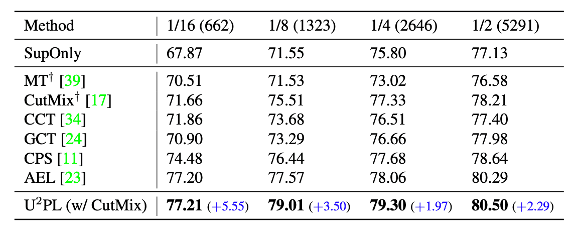
The comparison results between the semi-supervised learning methods and our method when the PASCAL VOC dataset is split are shown in the table below. The table shows that our method has the highest accuracy for all segmentation methods.

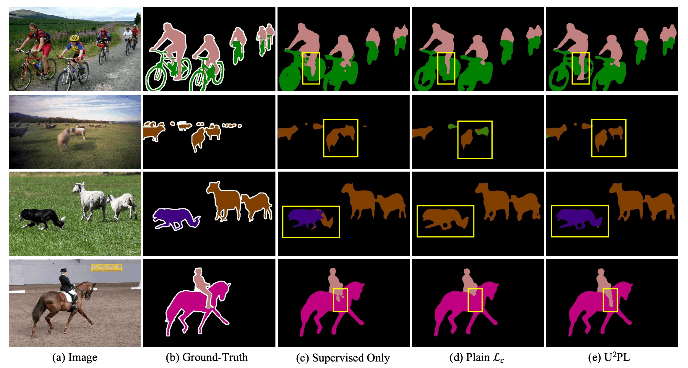
An example of the qualitative comparison result is shown in the figure below. From the figure, it can be seen that our method correctly predicts the areas where the model trained with only labeled data was incomplete.

summary

In this paper, we proposed a novel semi-supervised segmentation method, $U^2PL$, which exploits imprecise data. The proposed method shows better performance than the conventional semi-supervised methods. Compared with supervised learning, the disadvantage of semi-supervised learning is that it takes a lot of training time. However, it seems that time should be compensated for to achieve high accuracy without a large amount of label data.