New MDP For Highways! Extensible State Definition (Part 1)
3 main points
✔️ Planning (route planning) in driving
✔️ New MDP (Markov Decision Process) on highways
✔️ A combination of reinforcement learning and reverse reinforcement learning
Advanced Planning for Autonomous Vehicles Using Reinforcement Learning and Deep Inverse Reinforcement Learning
written by C You, J Lu, D Filev, P Tsiotras
(Submitted on 2019)
Comments: Robotics and Autonomous Systems 114 (2019): 1-18.
Subjects: Machine Learning (cs.LG); Machine Learning (stat.ML))
Introduction
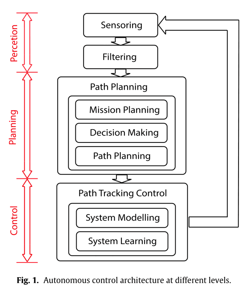
Accidents caused by driver error are becoming more frequent. For this reason, interest in automated driving is increasing. As shown in the following figure, there are three levels of automated driving: Perception, Planning and Control. This paper is a study of the planning part.
Contribution
The three main contributions of this paper are as follows
- New MDP models for highways
- The shape of the road is taken into account and can be easily expanded
- Remove the speed of the vehicle so that the state space is not too large
- Arbitrary nonlinear reward function with a generalization of Max Ent IRL
- Three Max Ent deep IRL proposals for model-free MDP
MDP stands for Markov Decision Process. In the first half of this article, we will introduce the proposed methodology. The second half of this article introduces the experiments and results. Now, let's look at the paper.
Traffic Modeling
Markovian decision-making process
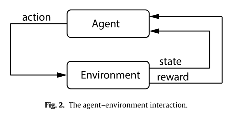
Let's start with a basic description of the Markov decision process. Markov decision processes are used in a wide range of fields, including robotics, economics, manufacturing, and automated driving. A Markov decision process is a mathematical framework for probabilistic modeling of the interaction between an agent and its environment. Agents receive rewards and representations (observations) of the state of the environment at each time step and act on them.
A typical Markov decision process consists of six tuples.
$$(S, A,{\cal T},\gamma, D, R)$$
- $S$: a finite set of possible states.
- $A$: a finite set of possible states.
- ${\cal T}$: State transition probability matrix (all state pairs)
- $\gamma$: Discount rate $\gamma\in [0,1)$
- $D$: Initial state distribution
- $R$: Reward function
Markov property is a property in which the future probability distribution depends only on the present and not on the past. In the equation, if $s$ is a state and $a$ is an action, it is a property satisfying the following equation.
$${\mathbb P}(s_{t+1}|s_t,a_t,s_{t-1},a_{t-1},...,s_0,a_0)={\mathbb P}(s_{t+1}|s_t,a_t) \tag{1}$$
The problem of the Markov decision process is to find the measure $\pi:S\rightarrow A$. The optimal measure can be defined by the following formula.
$$\pi^* = \arg\max_\pi {\mathbb E}\Biggl[\sum_{t=0}^\infty\gamma^t R(s_t,\pi(s_t))\Biggr] \tag{2}$$
And if we express the Markov property as an expression using the measure $\pi$
$${\mathbb P}^\pi(s_{t+1}|s_t)={\mathbb P}(s_{t+1}|s_t,\pi(s_t))\tag{3}$$
Systems modeling
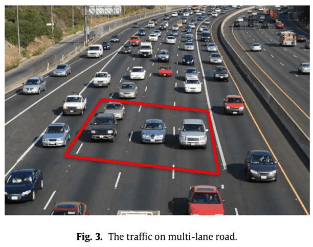
In this section, we model the Markov decision process for a highway scenario as shown in the following figure.
Let the vehicle under control be the host vehicle (HV) and all other vehicles be the environmental vehicles (EVs). The action set ${\cal A}$ is {"maintain speed", "accelerate", "decelerate", "turn left" and "turn right"}.
State definition
The state is represented by the following figure
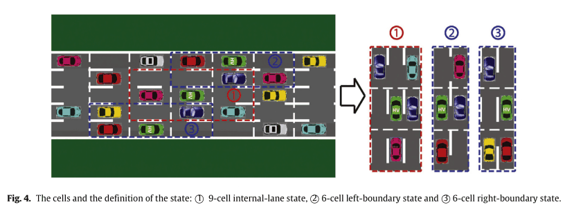
If you are in the center lane, you have nine cells, and if you are in either end of the lane, you have six cells to represent your state. The green car in the figure is the HV and the agent in this case. In this case, the number of Markov decision processes is $2^8+2\times 2^5=320$, counting the presence or absence of EVs around it, respectively. With this definition, we can easily expand it as the number of lanes (more than 2) and cars change.
In this case, we also consider curves like the one shown in the following figure.
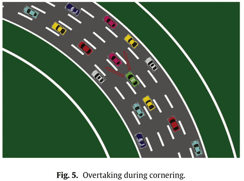
Since there is a difference between overtaking from the inside and overtaking from the outside in curves, we will consider three types of curves: straight lines, left curves, and right curves. In other words, the number of Markov decision processes is $320\times 3=960$.
Thus, further classifications can be made if necessary. For example, uphill, downhill and flat.
State Transition
The next step is state transitions. State transitions have the following assumptions
- The number of lanes $n$: $n\geq 2$
- The number of EVs $N$: $0\leq N\leq 8$
- EVs have their own measures that are different from HV
- EVs' actions are random.
- The EVs won't crash into HVs from the EVs.
- Each vehicle does one action at each time step.
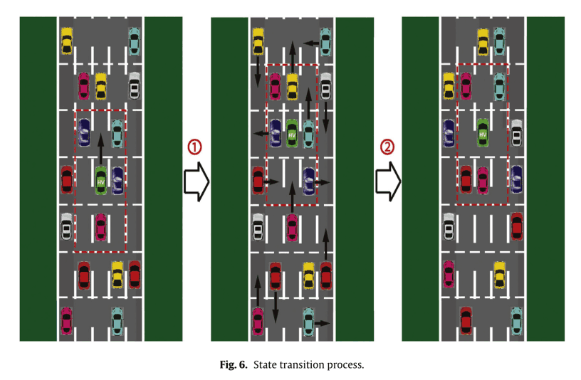
Based on the above assumptions, the transition from state $s_t$ to $s_{t+1}$ involves two steps.
- HV observes $s_t$ and acts according to the current measure $\pi(s_t)$
- EVs follow the behavior of HVs and behave randomly
In the example shown in the following figure, the safe action for HVs is to accelerate or change lanes to the left. In this case, acceleration is selected and the surrounding EVs take the safe random action accordingly.
Reinforcement learning
Selecting a reinforcement learning algorithm
The main reinforcement learning algorithms are tabular or functional approximation methods. Tabular forms are suitable for solving Markov decision processes in finite and small state action spaces. For example, dynamic programming, Monte Carlo methods and TD learning methods.
Traditional dynamic programming uses a value function to find the optimal measure. For example, value iterative and policy iterative methods. However, it requires full knowledge of the environment and cannot be used for continuous state action spaces. Monte Carlo methods do not require full knowledge of the environment. Instead, it requires a sample sequence of states, behaviors, and rewards for the agent's interaction with the environment. Episode-by-episode sample returns are averaged, i.e., the learning of values and corresponding measures takes place at the end of each episode. TD learning methods are a combination of dynamic programming and Monte Carlo methods, with the advantage that they do not require full knowledge of the environment and can be learned online. For example, Sarsa and Q-learning.
The difference between Sarsa and Q-learning is the future state action value that is referred to when updating the current state action value, Sarsa stands for "state-action-reward-state-action", which means that in order to update the action value in the current state, the action value in the next step The action value of the agent is used. In contrast, Q-learning searches for the maximum possible action value the agent can take in the next step and uses that value to update the action value in the current state. Thus, Sarsa is an on-policy algorithm and Q-learning is an off-policy algorithm.
Q-learning uses the ε-greedy method to easily trigger a 'death' in each episode, potentially providing a better strategy." Death" is the end of an episode when the episode reaches a certain state (the target state).
Functional approximations are used for large or continuous state-space problems and can represent values, measures, and rewards using a set of (nonlinear) functions. In theory, all methods used in the supervised learning domain can be used for reinforcement learning as function approximations. For example, neural networks, naïve Bayes, Gaussian processes, and support vector machines.
Since the model of the Markov decision process described in the previous chapter has a finite number of states and actions and the agent does not predict the behavior of EVs, we use a model-free method in tabular form.
Reward Functions
Next, let's talk about the reward function, which is important in reinforcement learning. Designing the reward function is a difficult task in the driving task because it is difficult to characterize the driver's behavior and the actual reward function is unknown. Moreover, the reward function may differ from one driver to another. A widely used method of designing a reward function is to represent it as a function of manually selected features. The features depend on the behavior of the agent and the state of the environment. In this article, we use a linear combination of features to represent the reward function.
$$R(s,a)=w^T\phi(s,a)\tag{4}$$
However, $w$ is a weight vector and $\phi$ is a feature vector.
This time, $\phi$ consists of the following five elements.
- behavioral characteristics
- HV location
- overtaking strategy
- joint ownership
- collision
In 1, the driver may prefer certain behaviours that are more rewarding; 2, whether the HV is driving close to the road boundary; 3, when passing in a corner, he may have a preference for passing from the inside or outside; 4, whether the HV is behind the EV; 5, whether the HV and the EV are in the same square. 5 is whether the HV and the EV are in the same square.
We use these feature takers to design a weight vector $w$ to encourage or punish a particular feature, and use reinforcement learning to learn the optimal strategy to maximize the total reward.
Another idea is to design the reward function using parameterized function approximators such as Gaussian processes or Deep Neural Netwark (DNN). The parameters of the function approximator may not be directly related to a clear physical meaning, so it is difficult to design them manually and learn them from the data.
The Maximum Entropy Principle and Reward Function
The approach in the previous chapter is inconvenient when there is insufficient prior knowledge of the reward function. Therefore, we use inverse reinforcement learning, which avoids manual design of the reward function and allows the user to learn the best driving strategy directly from the expert driver's demonstration.
maximum entropy principle
The maximum entropy principle has been used in many areas of computer science and statistics. In the basic formulation, given a set of samples from the target distribution and a set of constraints on the target distribution, the target distribution is estimated using the maximum entropy distribution such that the constraints are satisfied. In the inverse reinforcement learning problem, the agent's time history (demo), consisting of past states and behaviors, is given to estimate the reward function. The problem with previous inverse reinforcement learning was that the reward function was not uniquely determined, but by using the maximum entropy principle, the solution can now be uniquely determined. In the first Maximum Entropy Principle of Inverse Reinforcement learning (Max Ent IRL), the reward function depends only on the current state and is represented by a linear combination of feature functions.
$$R(s)=\sum_i w_i \phi_i(s)=w^T\phi(s)\tag{5}$$
The probability of demo $\zeta \triangleq \{s_0,a_0,...,s_T,a_T\}$ is
$${\mathbb P}(\zeta|w)=\frac{1}{Z(w)}e^{\sum_{s\in \zeta}w^T\phi(s)}\tag{6a}$$
$${\mathbb P}(\zeta|w)=\frac{1}{Z(w)}e^{\sum_{s\in \zeta}w^T\phi(s)}\prod_{(s,as')\in\zeta}{\mathbb P}(s'|s,a)\tag{6b}$$
Equation (6a) represents the definitive Markov decision process and Equation (6b) represents the stochastic Markov decision process. Both equations in Equation (6) show a distribution on the path (demo), where the probability of the path is proportional to the exponent of its reward. This means that paths with higher rewards are more desirable (more probable) to the agent. The goal of inverse reinforcement learning is to find the optimal weights $w^*$ such that the likelihood of the observed demo is maximized under the distribution of equation (6).
In the following, we will formulate the inverse reinforcement learning problem using a new reward structure.
- Using $R(s,a)$($\phi(s,a)$) instead of $R(s)$ ($R(s,a)$)
- Dealing with Probabilistic Markov Decision Processes
- The demo must start in the same state $s_0$ and is observed over a period of the same length of time from $t=0$ to $t=T$
notation
- $D$: A set of demos.
- $N$: Number of demos in $D$
- $Omega\supseteq$: Complete path space
- $\phi_\zeta$: The number of features along the path $\zeta \in D$
($\phi_\zeta = \sum_{(s,a)\in\zeta}$)
unparameterized feature
Let's first consider features that are not parameterized, i.e., not approximated by neural networks, etc. The unparameterized feature $\phi(s,a)$ is a function of state and behavior only. Using this, the reward function can be viewed as a linear combination of features of the following form
$$R(w;s,a)=w^T\phi(s,a) \tag{7}$$
We denote $R(w;s,a)$ to make it explicit that the reward function depends on an unknown weight vector $w$. From a related study [2], maximizing the entropy of the distribution on $\Omega$, which is affected by the feature constraint of the observed $D$, is the same as maximizing the likelihood of $D$ under the maximum entropy distribution in Equation (6b). In other words, the formula is as follows.
$$w^*=\arg \max_w {\cal L}_D(w)=\arg\max_w \frac{1}{N}\sum_{\zeta\in {\cal D}}\log{\cal P}(\zeta|w)\\ =\arg \max_w \frac{1}{N}(\sum_{\zeta\in{\cal D}}(w^T\phi_\zeta + \sum_{(s,a,s')\in\zeta}{\mathbb P}(s'|s,a)))-\log Z(w) \tag{8}$$
parameterization feature
Using unparameterized features requires designing features manually, but it is not always possible to successfully design unknown reward functions with complex forms. In general, this is a difficult task. Therefore, we use parameterized features. By using parameterized features, we avoid designing features manually by optimizing the parameters. to formulate the Max Ent IRL problem, we consider a reward function represented by a linear combination of features, but the features depend explicitly on the parameter $\theta$.
$$R(w,\theta;s,a)=w^T\phi(\theta;s,a) \tag{9}$$
Instead of adjusting only the weights $w$ in equation (8), we also adjust $\w$ and maximize the likelihood ${\cal L}_D$ as follows
$$w^*,\theta^*=\arg\max_{w,\theta} {\cal L}_D(w,\theta)=\arg\max_{w,\theta}\frac{1}{N} \sum_{\zeta\in {\cal D}}\log {\mathbb P}(\zeta | w,\theta)\\ =\arg\max_{w,\theta} \frac{1}{N} (\sum_{\zeta\in {\cal D}}(w^T\phi_\zeta(\theta)+\sum_{(s,a,s')\in\zeta}{\mathbb P}(s'|s,a)))-\log Z(w,\theta)\tag{10}$$
The figure below shows the parameterization process.
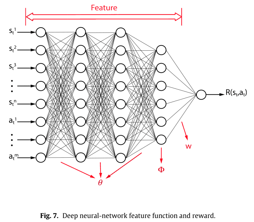
Here, setting $w=1$ allows us to represent the reward function directly using a single DNN, and the maximum entropy distribution across the path space $\Omega$ is obtained by adjusting only for $\theta$.
Reverse reinforcement learning
compensation approximator
We use the DNN as a function approximator to recover unknown rewards. We also consider three definitions of reward functions from related studies.
- $R$: $S\rightarrow R$, $R(s)$
- $R$: $S\times A\rightarrow R$, $R(s,a)$
- $R$: $S\times A\rightarrow R$, $R(s,a,s')$
The first definition is used when you want to reach a goal state without an action, or to avoid a dangerous situation. This definition indicates that the agent has no special behavior for the action.
The second definition considers behavior and thus allows us to express the agent's preference for a particular behavior.
The third definition also considers the next state $s'$ after executing the action $a$ in state $s$. However, $s'$ depends on the response of the environment, and the agent can decide to act according to the expected reward for performing the action $a$ without knowing the future state. Thus, $R(s,a)$ and $R(s,a,s')$ can be said to be equivalent.
For these reasons, we will use $R(s,a)$ in this case.
There are two possible structures of DNNs to represent $R(s,a)$, as shown in the following figure.
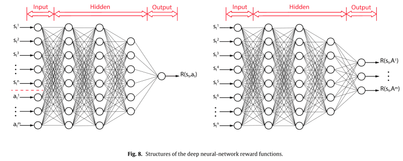
Maximum Entropy Inverse Reinforcement Learning
The IRL algorithm used for learning the parameters in Fig. 8. is explained using the maximum entropy principle of the previous section.
Model learning
Consider a completely model-free case with no knowledge of the state transition model ${\mathbb P}(s'|s,a)$. The idea of model training is to analyze the number of visits for each state-behavior-state and compute the probability of state transitions.
$${\mathbb P}(s'|s,a) = \frac{\nu(s,a,s')}{\sum_{s'\in S}\nu(s,a,s')} \tag{11}$$
However, $\nu(s,a,s')$ is the total number of state transitions from $s$ to $s'$ when an action $a$ in state $s$ is performed. As $\nu(s,a,s')$ approaches infinity, the probability ${\mathbb P}(s'|s,a)$ approaches the actual value.
The model is taught through Q-Learning.
Inverse reinforcement learning algorithm
First, we calculate the expected state - the number of action visits ${\mathbb E}[\mu(s,a)]$ by using the result of model training ${\mathbb P}(s'|s,a)$. Based on that, calculate $\frac{\partial\Partial L}_D}{R}$. Using that, calculate $\frac{\partial{\cal L}_D}{\partial \theta}$ and update the parameters according to the following formula.
$$\Delta\theta = \lambda\frac{\partial{\cal L}_D}{\partial \theta}\tag{12}$$
Improved inverse reinforcement learning algorithm
Training the model may not yield good results in front of a large number of visits per state-behavior pair. This is due to the following accumulation of errors.
The error of state transition probability ${\mathbb P}(s'|s,a)$ → The error of $\frac{\partial{\cal L}_D}{\partial R}$ → The error of $\frac{\partial{\cal L}_D}{\partial \theta}$ at the time of update of $\theta$
Here are two ways to respond to this.
- Pre-training the model until it converges before reverse reinforcement learning
- Divide the demo into smaller pieces to avoid large errors due to long-term predictions
The first is that, although an improvement is possible, the demo ${\cal D}$ may still be insufficient to represent the random behavior of the environment if the system is complex or if the entire demo represents the long-term behavior of the stochastic system.
This time we will use the second strategy. Divide the demo ${\cal D}$. $$\cal D_\tau = \zeta_\tau^i\,i=1,...,N_\tau$$
There are three division rules.
- $\zeta_\tau^i$ starts from $\tau\in S$.
- The length of $\zeta_\tau^i$ is constant in $\Delta T$ with respect to all $\tau\in S$.
- Pathway $\zeta\in {\cal D}$ such that $\zeta_\tau^i\subseteq \zeta$
The path space corresponding to $\zeta_\tau$ is represented as $\Omega_\tau$ and maximizes the entropy of the contemporaneous distribution across all $\Omega_\tau$, constrained by the demo ${\cal D}_\tau$.
Conclusion
What do you think? In the first half of this article, we have introduced the proposed methodology. The proposed MDP (Markov Decision Process) traffic model is attractive because it is easy to extend. We extended the reward function $R(s)$, which is unsuitable for complex tasks because it only considers states in inverse reinforcement learning, to $R(s,a)$. This is the first time this generalization has been made in this paper. In the second half of this paper, we will present our experiments and results. Please refer to the second half of the paper.
References
[1] You Changxi, Jianbo Lu, Dimitar Filev, Panagiotis Tsiotras. "Advanced planning for autonomous vehicles using reinforcement learning and deep inverse reinforcement learning." Robotics and Autonomous Systems 114 (2019): 1-18.
[2] E.T. Jaynes, "Information theory and statistical mechanics", Phys. Rev. 106 (4) (1957) 620–630.


Categories related to this article