New MDPs For Highways! Extensible State Definition (Part 2)
3 main points
✔️ Planning (route planning) in driving
✔️ New MDP (Markov Decision Process) on highways
✔️ A combination of reinforcement learning and reverse reinforcement learning
Advanced Planning for Autonomous Vehicles Using Reinforcement Learning and Deep Inverse Reinforcement Learning
written by C You, J Lu, D Filev, P Tsiotras
(Submitted on 2019)
Comments: Robotics and Autonomous Systems 114 (2019): 1-18.
Subjects: (Machine Learning (cs.LG); Machine Learning (stat.ML))
Introduction
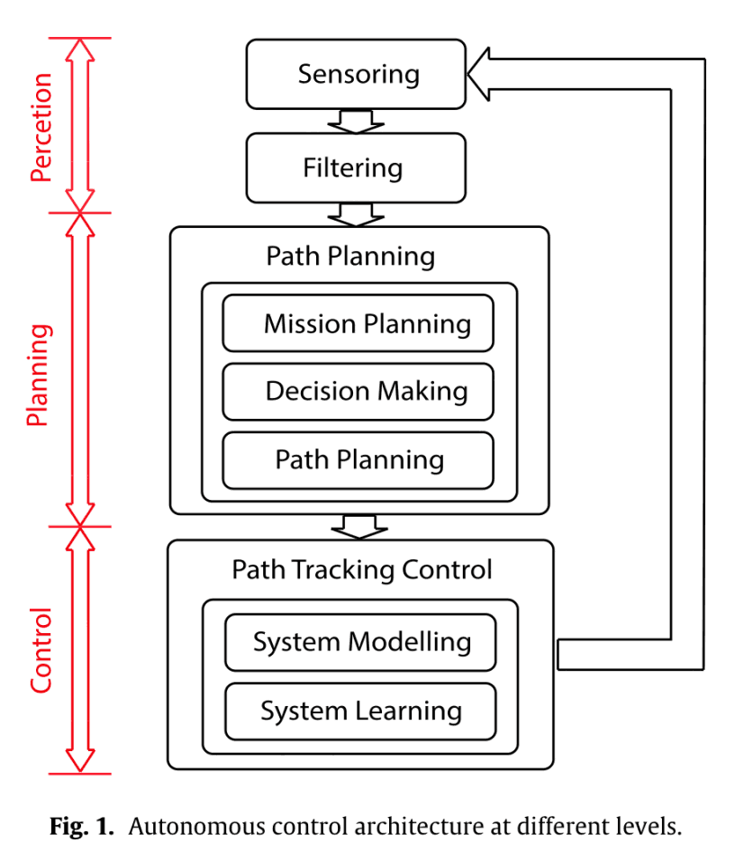
Accidents caused by driver error are becoming more frequent. For this reason, interest in automated driving is increasing. As shown in the following figure, there are three levels of automated driving: Perception, Planning and Control. This paper is a study of the planning part.
Contribution
The three main contributions of this paper are as follows
- New MDP models for highways
- The shape of the road is taken into account and can be easily expanded
- Remove the speed of the vehicle so that the state space is not too large
- Arbitrary nonlinear reward function with a generalization of Max Ent IRL
- Three Max Ent deep IRL proposals for model-free MDP
MDP is a Markov Decision Process. In the previous article (part 1), I explained the proposed method. We defined a new MDP (Markov Decision Process) for traffic models of highways and proposed an extension of maximum entropy inverse reinforcement learning.
Now, let's look at the experiment.
Experiments, Results, and Analysis
In this chapter, we will implement the reinforcement and inverse reinforcement learning algorithms on the traffic model described and analyze the results.
Traffic simulator
This is the content of the simulator used in this experiment, which was created using the Python library called Pygame. The number of lanes is 5. The vehicle type (truck, sedan, etc.) is not distinguished. Each EV has a random strategy. The random strategy uses all the surrounding vehicles (HVs and EVs) to define the state $s_{EV}$, find a set of actions that will not cause the EVs to collide, and then randomly determine an action from that set.
Setting driving behavior through reinforcement learning (expert)
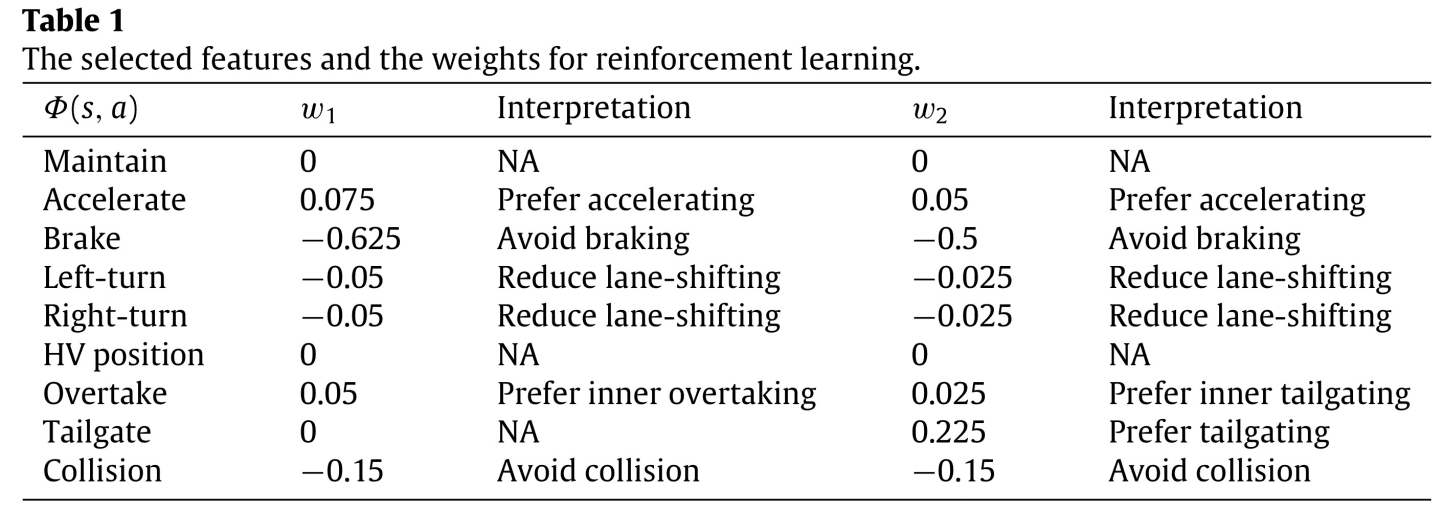
Here, you will use reinforcement learning to acquire expert driving behaviors. In this case, we have two types of weights: overtaking and following. The designed weights $w_1$ (overtaking) and $w_2$ (following) are shown in Table 1.
The desired driving behavior (overtaking) by the design of $w_1$ is as follows.
- If the cell in front of the HV is free, the HV accelerates and occupies the cell in front of it.
- If there is an EV in front of the HV and cannot pass, the HV maintains its speed.
- When only one side of the car can pass, the HV overtakes the EV in front by first changing lanes, accelerating, and then holding the speed.
- HVs overtake from the inside of a corner when they can pass from both sides.
- HVs don't change lanes unless they are passing.
- HVs do not occupy the rear cell by applying the brakes.
- Conflicts are not allowed.
The desired operation behavior (follow-up) by the design of $w_2$ is as follows
- When an EV is in front of an HV, the HV maintains its speed.
- The HV accelerates to occupy the cell in front of the vehicle when the cell in front of the vehicle is empty and a lane change does not cause it to follow.
- When there is no EV in front of the HV, the HV changes lanes to follow the EV.
- HVs prefer to follow vehicles in the lane inside the corner.
- HVs do not change lanes unless they follow.
- HVs do not occupy the rear cell by applying the brakes.
- Conflicts are not allowed.
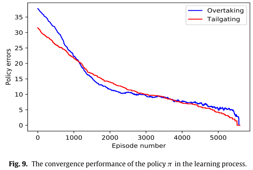
We used Q-learning to learn these optimal strategies. $w_1$: $w_1^*$ and $w_2$: $w_2^*$ corresponding to $w_1$: $\pi_1^*$. The next figure shows the convergence.
Here is an example of the results of a simulation using the policy $\pi_1^*$.
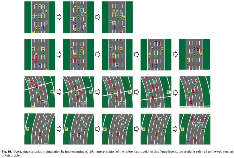
The first line is a scenario where there is space in front of the HV; the HV accelerates and is behind the yellow vehicle.
The second line is a scenario where there is one vehicle in front of the HV and both left and right lanes are available for overtaking. Since the road is a straight line, you can overtake from either side. In this case, the car overtakes from the left and accelerates until it catches up with the blue car.
The third line is a scenario with vehicles in front of and to the right of the HV; the HV can only use the left lane to pass.
Line 4 is a scenario where there is one car in front of the HV and both left and right lanes are available for overtaking. The car changes lanes to the right, inside the corner, and accelerates, but does not complete the pass because the cyan car also accelerates.
These behaviors are consistent with the behaviors we aimed for in the design of the weights $w_1$ and have been successfully learned.
Acquisition of Driving Behaviors through Reverse Reinforcement Learning
First, we implement $\pi_1^*$ and $\pi_2^*$ to learn the reward function represented by a DNN, and then use the maximum entropy principle to obtain the estimation measures ${\hat\pi}_1^*$ and ${\hat\pi}_2^*$. First, we select the structure of the DNN in Fig. 8. to represent the reward function. In this case, we used the second one, which is more convenient. The state vector $s_t$ is 10 dimensions of the positions of the nine vehicles (1 HV and 8 EVs) and the road types. There are five actions in $A$. They are speed maintenance, acceleration, deceleration, lane change right, and lane change left. The initial state of the simulation $s_0$ is shown in Fig. 11. There are three EVs around the HV, in the middle lane of the 5-lane road. The simulation duration $T$ is 1500 and the number of demonstrations is 500.
Next, we implemented three types of maximum entropy inverse reinforcement learning, Algorithm 4 is conventional maximum entropy inverse reinforcement learning, and Algorithms 5 and 6 are maximum entropy inverse reinforcement learning of the proposed method. The difference is the duration of the split $\Delta T$. The results are shown in Table 2.

Table 2 shows that the traditional method, Algorithm 4, does not converge. This is due to the long data length and probabilistic behavior of the system. The proposed Algorithm 5 and 6 converge, but the computation time is shorter than that of Algorithm 6 because Algorithm 5 does not calculate the expected value of the number of visits of the state-action pair since $\Delta T =1$.
We also implemented the learned measures ${\hat\pi}_1^*$ (overtaking) and ${\hat\pi}_2^*$ (following) in the simulation. Since ${\hat\pi}_1^*$ was the same as $\pi_1^*$, it is the same as Fig. 10. Fig. 12. shows ${\hat\pi}_2^*$ as shown in Fig. 12.
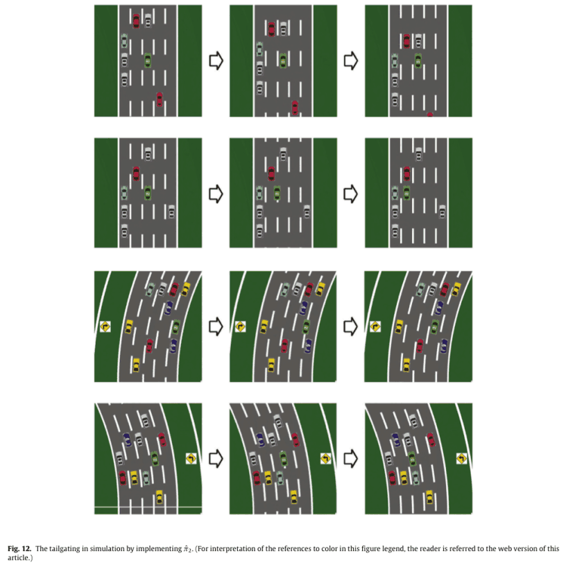
The first line is a scenario where there is space in front of the HV; the HV cannot follow the EV by changing lanes, so it accelerates to fill the space in front of it.
The second line is a scenario in which the HV changes lanes to the left to follow.
The third line is similar to the second line, but is a cornering scenario.
In line 4, the HV can follow the left side of the road by changing lanes on either side, but it prefers to follow the left side of the curve.
These actions are consistent with the actions aimed at in the design of the weights $w_2$, and we can say that we have successfully obtained the measure from the measure $w_2$.
Conclusion
A stochastic Markov decision process was used to model traffic and reinforcement and inverse reinforcement learning was used to achieve desired driving behavior. State and MDP traffic model definitions are flexible and can model traffic for an arbitrary number of lanes and an arbitrary number of EVs. Driving strategies may change depending on the curves in the road and can be taken into account. Although the state definition scales easily and solves the MDP problem efficiently, the model does not distinguish between different vehicle speeds or vehicle types and treats each vehicle as a quality point. Additional work is needed to use the results of this paper in a real-world scenario. For example, dynamically changing the magnitude of the MDP state depending on the (relative) speed in traffic. The design of the driver's reward function allowed us to use Q-learning to learn the corresponding optimal strategy and to demonstrate typical driving behaviors such as overtaking and following.
To recover measures and reward functions from the data, we proposed a new model-free inverse reinforcement learning method based on the maximum entropy principle. Most of the existing methods are $R(s)$, but we used $R(s,a)$, which can design a more diverse range of behaviors. It is the first generalization of maximum entropy inverse reinforcement learning with arbitrary parameterized, continuously differentiable function approximations (DNNs).
We have shown that it is difficult to use long demonstrations for IRL when the knowledge of probabilistic systems is limited.
Errors arise from two main factors.
- If the amount of data is not sufficient to represent the stochastic behavior of the system
- If the prediction error of a stochastic system accumulates and becomes large over time in a model-free problem
In contrast, we improved the IRL algorithm by dividing the demo into shorter data pieces and maximizing the entropy of the contemporaneous distribution on the data pieces.
The proposed methodology was validated by simulation.
Summary
Future directions include high-fidelity simulations, designing controllers in real-world tasks, the introduction of partial observation MDPs for decision making with imperfect perception, and the introduction of multi-agents for better control of traffic flows. It would be interesting to use the present method in simulations using CARLA etc. . It is also necessary to deal with imperfect perception in driving, because it is said that it exists. Although this paper was not an end-to-end approach to driving, the new MDP is very attractive because it can be extended. If it could be used as an adjunct to the planning of other end-to-end methods, it might help to prevent accidents and reduce traffic congestion. Although it may be difficult to use this method in real-world tasks as it is, it would be interesting to use it like a navigation command and combine it with control.
References
[1] You Changxi, Jianbo Lu, Dimitar Filev, Panagiotis Tsiotras. "Advanced planning for autonomous vehicles using reinforcement learning and deep inverse reinforcement learning." Robotics and Autonomous Systems 114 (2019): 1-18.
[2] E.T. Jaynes, "Information theory and statistical mechanics", Phys. Rev. 106 (4) (1957) 620–630.


Categories related to this article