
BILCO For Accurate And Fast Alignment Of Time Deviations Between Time Series Data Series
3 main points
✔️ NeurIPS 2022 Accepted paper, BILCO aligns time series data when there is a time shift between series
✔️ Traditional joint alignment methods are accurate, but computationally expensive and not widely used
✔️ Ingenious initialization and a bi-directionalPushing strategy convert the original problem into two smaller subproblems, resulting in an average speedup of 20x
BILCO: An Efficient Algorithm for Joint Alignment of Time Series
written by Xuelong Mi, Mengfan Wang, Alex Bo-Yuan Chen, Jing-Xuan Lim, Yizhi Wang, Misha Ahrens, Guoqiang Yu
(Submitted on 01 Nov 2022)
Comments: NeurIPS 2022 Accept
The images used in this article are from the paper, the introductory slides, or were created based on them.
summary
This is a NeurIPS 2022 accepted paper. When dealing with time-series data, time shifts occur between multiple time-series data, and alignment is one of the fundamental preprocessing steps in data analysis. Traditional pairwise alignment methods have been used, but these time series data are often interdependent and do not make good use of this information as it adds extra information to the alignment task. Recently, joint alignment has been modeled as a max-flow problem, where the profile similarity between aligned time series and the distance between adjacent warping functions are jointly optimized. However, despite its elegant mathematical formulation and excellent alignment accuracy, this new model, which uses an existing general-purpose max-flow algorithm, is computationally time-consuming and memory-intensive, which are major constraints on its widespread adoption. This paper presents BIdirectional pushing with Linear Component Operations (BILCO), a new algorithm that efficiently and accurately solves the joint alignment maxflow problem. Here we develop a strategy for linear component operations that integrates dynamic programming and a push-label approach. The strategy is motivated by the fact that the joint alignment max-flow problem is a generalization of dynamic time warping (DTW), in which many individual DTW problems are embedded. Furthermore, taking advantage of another fact that good initialization can be easily computed for the joint alignment max-flow problem, a bidirectional pushing strategy is proposed to introduce prior knowledge and reduce unnecessary computations.
The demonstrability of BILCO was verified using both synthetic and real-world experiments, and tested on thousands of data sets in a variety of simulation scenarios and three different application categories, showing that BILCO consistently achieves at least 10x and on average 20x and consistently achieves speedups of at least 10x and on average 20x and memory usage of up to 1/8 and on average 1/10, respectively, compared to the best existing maxflow methods.
Introduction.
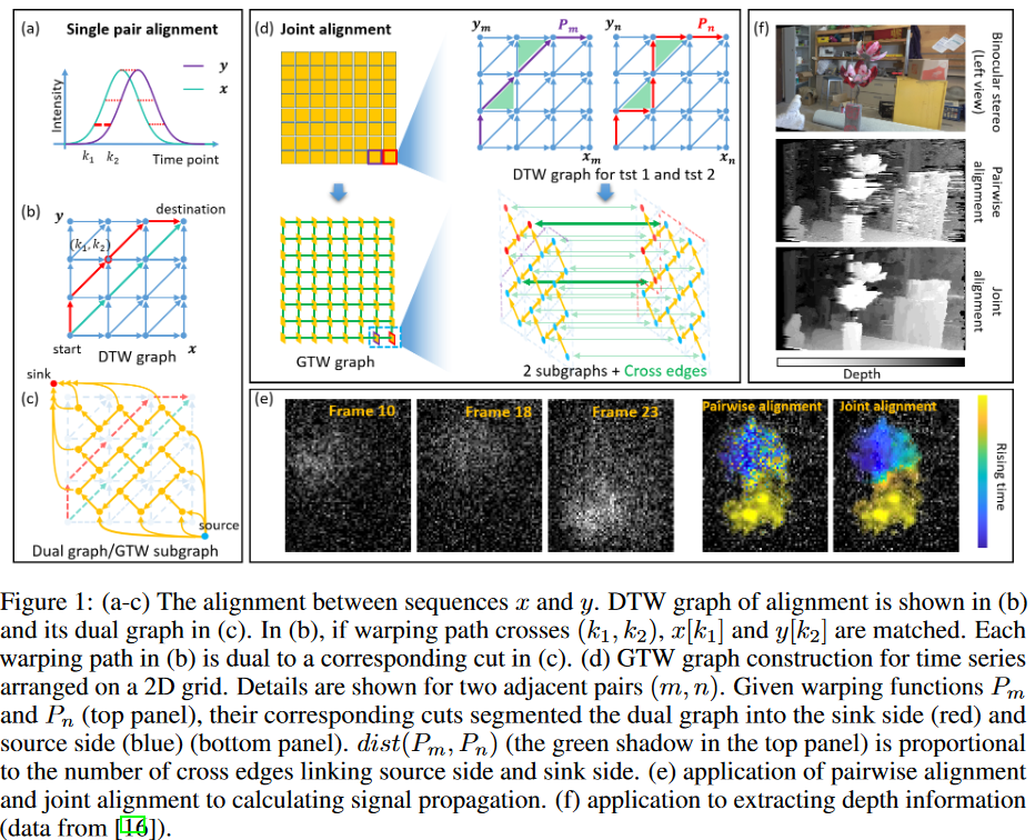
Time series data naturally appear in a variety of fields, such as motion capture, speech recognition, and bioinformatics. Time-series data usually cannot simply be directly compared between data series or points in time due to the possibility of delays and distortions, so alignment between data is an essential pre-processing step. The most common alignment method, dynamic time warping (DTW), uses dynamic programming (DP) to find the best match between two sequences in linear time. However, DTW and its variants only compare a single pair of time series and do not take advantage of the structural information contained in the real data. For example, in time-lapse microscopy data, pixel intensities are recorded over time on a two-dimensional grid, and neighboring pixels tend to have similar temporal patterns. Therefore, joint alignments of more than a single pair are expected to achieve better performance by exploiting dependencies from the structure.
For a long time, it was not clear how to incorporate structural information in principle, but various heuristic tricks have recently been developed. In a recent theoretical breakthrough, the joint alignment problem was elegantly modeled as a max-flow problem for graphical time warping (GTW) graphs by optimizing both the time series pairwise similarity and the distance between warping functions. GTW has been used in brain activity analysis and It has been shown to have excellent alignment accuracy in many applications such as liquid chromatography-mass spectrometry (LC-MS) proteomics, where the warp function represents the delay of the real signal at each time point relative to a reference time series, and adjacent time series should propagate similarly. By adding a penalty to the dissimilarity of the warp function, GTW can exploit the structural information and obtain better alignment performance, as shown in Fig. 1(e) and (f). However, GTW is solved with an existing general-purpose max-flow algorithm, which is computationally time-consuming and memory-intensive, limiting its wide application. In fact, for a typical dataset of 5000-time series, each containing 200-time points, incremental breadth-first search (IBFS), Hochbaum's pseudo flow (HPF), Boykov-Kolmogorov (BK ) max-flow, highest-label push-relabel (HIPR), etc., all common methods can consume several hours and over 100 Gbytes of memory.
In this paper, we identify two important properties of the joint alignment maxflow problem and show how they can be exploited to design new algorithms that improve both speed and memory efficiency. Specifically, first, joint alignment is a generalization of pairwise alignment, in which several individual DTW problems are embedded, as shown in Fig. 1(a)-(d). If the dependencies are ignored, the problem reduces to several independent DTW problems, which can be solved in linear time by DP. Although the dependencies make the problem more complex, the properties of the DTW problem can be exploited. Second, coarse approximate solutions for joint alignment can be easily estimated for many applications. Such prior knowledge can be incorporated to accelerate the max-flow algorithm.
Using these two properties, this paper develops a new algorithm, BIdirectional pushing with Linear Component Operations (BILCO), which accurately and more efficiently solves the joint alignment max-flow problem. The algorithm consists of two main strategies:
(a) Excess pushing with Linear Component Operations (ELCO), which exploits the first property and integrates the DP and push-relabel l approaches.
Each component is defined as a small subgraph containing connected nodes and their associated edges. Components are determined automatically and adaptively; by combining DP and subgraph properties, we show that all operations on each component can be accomplished in linear time. Linear component operations allow ELCO to achieve higher efficiency than the common push-relabel approach.
(b) Design a two-way push strategy that exploits the second property and uses prior knowledge as initialization.
This strategy simplifies the original problem into two smaller subproblems with opposite pushing directions. Although ELCO is applied in each problem, the separation of the two pushing directions dramatically reduces unnecessary computations.
BILCO has the same theoretical time complexity as the best general methods such as HIPR but provides significant empirical efficiency gains without sacrificing accuracy in the joint alignment task. Its effectiveness has been demonstrated through both synthetic and real-world experiments: comparing IBFS, HPF, BK, and HIPR with thousands of data sets from various simulation scenarios and three real applications in different categories, BILCO outperforms the best comparable methods by 10 to 50 times faster and at an average of one-tenth the memory cost.
problem definition
The time-series clause alignment problem can be formulated as follows
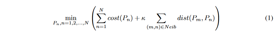
Pn denotes the warping path of the nth time-series pair, N is the total number of time-series pairs to be jointly aligned, cost(Pn) is the alignment cost of the nth time-series pair, and dist(Pm, Pn) is the warping path distance defined as the area of the region enclosed by Pm and Pn. a set of pair indices (m, n) representing adjacent time series, and κ is a hyperparameter to balance the alignment cost term and the distance term. For example, for 2-D grid time series data, Neib contains pairs of adjacent pixels and κ represents the prior similarity between pixels.
As shown in Fig. 1, Equation (1) can be solved by transforming it into a flow network and finding its min-cut. The constructed graph, the dynamic time-distortion methodGTW graph, consists of N GTW subgraphs {Gn = (V n, En)|n = 1, 2, ..., N } and a crossing edge Ecross of capacity κ2 (Fig. 1(d)); an edge in a GTW subgraph is called Ewithin. In the following content, we will refer to a GTW subgraph as a "subgraph" for convenience. Each subgraph Gn is dual to a DTW graph, which represents warping between a pair of time series. Since cuts in a subgraph are dual to the warping path of a time-series pair (Fig. 1(b)-(c)), a mini-cut in one DTW graph can be solved in linear time by finding the shortest path using dynamic programming (DP ). The cross-edges constrain the difference between cuts in adjacent subgraphs and correspond to the distance term in Eq. (1) (Fig. 1(d)). To guarantee the monotonicity and continuity of the warping path, the capacity of the inverse edge of each subgraph is set to infinity.
It is worth noting that the GTW framework is flexible and widely applicable and can be used as a building block to solve many problems while leveraging structural information. The assumed neighborhood structure and similarity strength can be application-specific or user-designed. For example, for different pairs of warping functions, GTW can be configured with different hyperparameters κ. For simplicity, the same hyperparameter κ will be used below for all pairs of warping functions in this paper.
technique
BILCO contains two main parts, ELCO and bidirectional pushing, respectively, as described above. Based on the initialization of the warping function, the bidirectional pushing strategy transforms the maximum flow problem into two subproblems, each of which is solved with ELCO. This integration leads to BILCO, which is then analyzed for time complexity and memory usage.
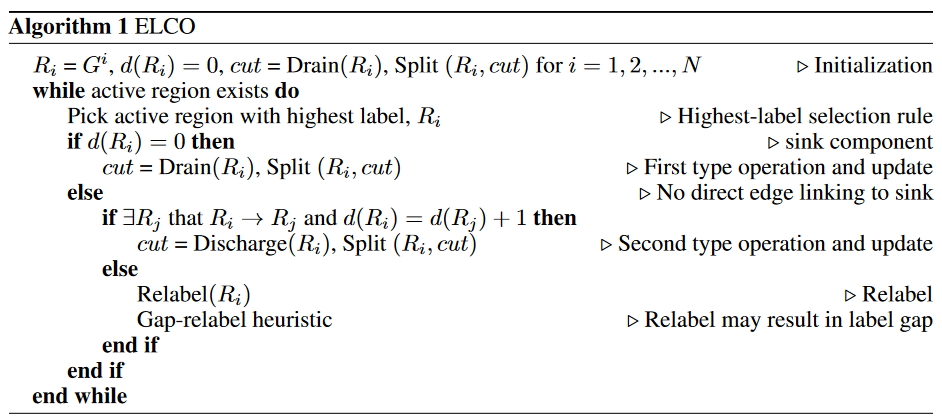
Excess pushing with linear component operations (ELCO)
Since GTW graphs contain many subgraphs that are dual to DTW graphs and each DTW graph can be solved linearly by DP, we expect the approach in this paper to make use of DTW graphs and the DP algorithm. Although the cross-edges between graphs preclude the direct use of DP, we find that the defined components are the largest subgraphs that allow the use of DP. By combining our newly devised graph transformation strategy (Fig. 3) with DP, we have established that the operations "Drain" and "Discharge" on the defined components can indeed be implemented linearly. To guarantee global optimality, we designed a new labeling function as shown in Section 3.1.4, which we use to guide the operations of the components.
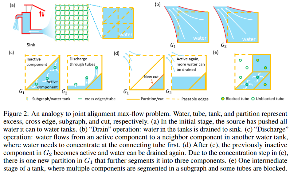
The basic unit of operation is not a node or subgraph, but a component
To exploit the properties of each subgraph, ELCO borrows the idea of a general push-label algorithm whose operations are localized; ELCO allows for the existence of a surplus, which is the surplus between incoming and outgoing flows of a single node. A node with a surplus is considered "active". Based on where the flows are exchanged, two operations are defined: "Drain" and "Discharge." "Drain" is an operation that pushes the surplus through Ewithin to the sink and is an operation in the subgraph. On the other hand, "Discharge" is a cross-subgraph operation that pushes the surplus out to the adjacent subgraph through Ecross. By alternating these two operations, more surplus can be sent to the sink (Fig. 2). As the surplus spreads, many edges become saturated, resulting in multiple cuts in the same subgraph. These cuts divide the subgraph into different components (Fig. 2(e)). We define a component as a subset of the GTW subgraph bounded by two adjacent cuts; ELCO uses components as the basic arithmetic unit instead of nodes or subgraphs. This is because the component is the largest unit when pushing a flow using DP.
Supplement 1
If two nodes are in the same component, there is at least one path connecting them.
By Supplement 1, if one node in a component is active, its surplus can spread anywhere in the same component. Thus, the entire component can be viewed as a single unit. Conversely, a cut interrupts flow across components in the same subgraph, so the entire subgraph cannot be viewed as a single unit.
With the component as the basic arithmetic unit, ELCO is described as follows. Initially, each subgraph is one active component. The "Drain" operation sends the largest remainder directly to the sink through Ewithin. A new cut is generated, blocking the surplus of the divided components closer to the source. Next comes the turn of Discharge, which looks for opportunities to move the surplus throughout the subgraph toward components that can perform the "Drain" operation. By alternating the operations of these two components, a global maximum flow can be achieved.
Linear time implementation of "drain" component operation
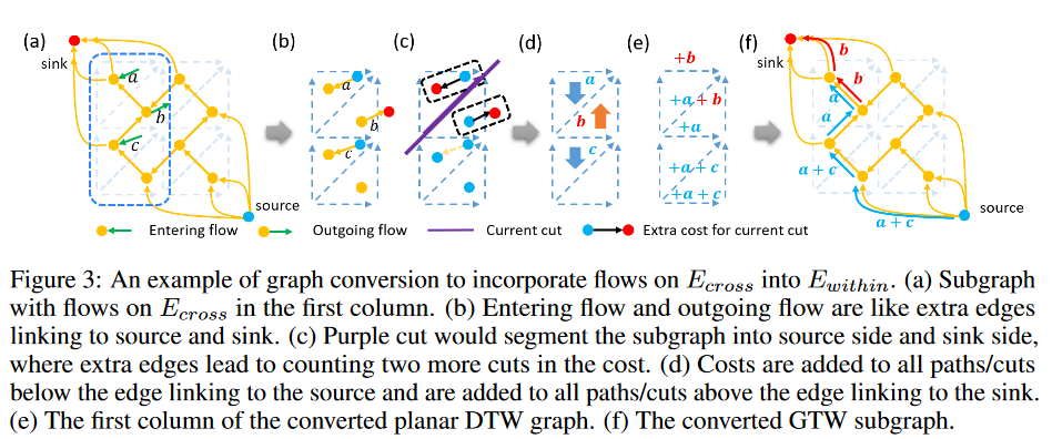
For the "drain" operation, one only needs to compute the min-cut of one active component linked to the sink and any excess above the new cut is drained, and the portion below the new cut is identified as the new active component (Fig. 2(b)(c)). As mentioned earlier, min-cut can be solved fast by DP on its dual graph. However, DP cannot be applied directly to flows on Ecross. The graph is no longer planar (Fig. 3(a) and (b)) and its dual graph does not exist. Therefore, we design a linear-time graph transformation strategy as shown in Fig. 3 (see Algorithm in the Supplement), which takes the known flows on Ecross into Ewithin and allows us to obtain an equivalent planar graph to which DP can still be applied. By combining the linear transformation strategy with DP, the "Drain" component operation can be realized in linear time.
Supplement 2
The corresponding cut value/path cost is the same before and after the graph transformation
Linear-time implementation of "discharge" component operation
To discharge one component, push out as much of the surplus as possible at each node, making sure the component has sent all of its surpluses. This is because surplus can flow anywhere within the same component.
Supplement 3
The maximum possible exceedance of node v is the min-cut value of the residual graph when v is the sink
Working with a modified DTW graph, DP can still compute such an excess by finding the difference between the shortest path below v and the shortest path of the entire graph. This difference can represent the min-cut value described in Supplement 3. To implement the "discharge" operation for the linear complexity component, we use another layer of DP that reuses a stored dynamic matrix that recursively stores the shortest distance.
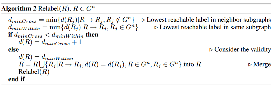
New labeling feature that directs excess material approaching the sink between components
This paper designs a new labeling function to derive the excess proximity t between components from high to low labels. Unlike the common push-relabel one, the labeling function here refers to the distance from a component to a sink, not from a node. Only Ecross is counted since the cut cuts off connections between components of the same subgraph. Derived from such distances, we define the labeling function d: V → N to be valid for all residual edges if

Supplement 4
All nodes of the same component have the same label
Supplement 5
The new labeling function (2) is consistent with the general push relabeling function if each component is treated as a single unit
Complement 4 suggests that one component and all nodes within it can be assigned the same label. Complement 5 suggests that ELCO can be viewed as an alternative push-label approach where the component is the unit of operation and that all statements of the general push-label approach hold at the component level as well. Since the validity of the labeling function is preserved in ELCO, the optimal solution can be achieved with polynomial component operations.
ELCO is outlined in Algo.1 and Algo.2, where R is the symbol of the component R1 → R2 applies the best label selection rule if (v, w) has positive residual capacity for v ∈ R1 and w ∈ R2, and both the global and gap relabeling heuristics are for acceleration.
Two-way push strategy
Typical push-label schemes and ELCOs try to push as much of the excess into the sink as possible. If some of the excesses cannot reach the sink due to edge capacity limitations, they must be absorbed by the source, which can take a long time and have high computational costs. Such a calculation is redundant because such a surplus cannot affect the maximum flow rate or change the final cut; ELCO reduces some of the redundancy within each component through linear component arithmetic, but it does not solve the problem between components, especially when κ is large (Ecross capacity is large) It cannot; when κ is large, Ewithin is more likely to saturate and the components are more likely to be split into smaller pieces. Thus, it is difficult to reduce redundancy by focusing only on each component.
As an extreme example, consider the case where all nodes are split into source-side VTs according to the cut. In this case, all the remainders can reach the sink and all push operations are not redundant. In the other extreme case, all nodes belong to the source-side VS. Most of the extras cannot reach the sink, but are still pushed, resulting in redundant computation. Conversely, it is a better strategy to push shortages from the sink than to push excess from the source. A deficit means that the input flow is less than the output flow. Pushing out a deficit is nothing more than pushing out an excess in a graph with a calculation. If one has the prior knowledge to find the initialization of the warping path, one can simply push out the excess on the sink side and the deficit on the source side. After that, there is very little computational waste. With this in mind, we decided to design a bidirectional pushing strategy (Fig. 4) in which the source and sink are swapped. Since all nodes are split into VSs, any operation that pushes the deficit in the opposite direction is not redundant. In conclusion, pushing an excess at the sink-side VT and a deficit at the source-side VS does not invalidate the graph.
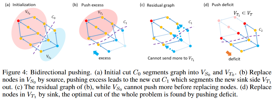
Initialization: Estimate the initial cut C0 of the GTW graph. Let VS0 and VT0 be the corresponding source and sink sides, respectively.
Extrude the excess: solve the max-flow problem by replacing all nodes in VS0 with sources and extruding the excess. Let VT1 be the new sink side divided by the new mini-cut C1.
Push in the red: replace all the nodes in VT1 with sinks and solve the max-flow problem with a push in the red. The resulting mini-cut C2 is a mini-cut of the original GTW graph.
This strategy is guaranteed to achieve the optimal solution by the following statements
Supplement 6
Assuming that the mini-cut splits node V into source-side VS and sink-side VT, replacing a VS or VT node with a source or sink does not affect the mini-cut.
Supplement 7
Let VT denote the sink-side node into which the real mini-cut of the original GTW graph is split, then VT1⊆ VT.
Theorem 1
The mini-cut obtained by the bidirectional strategy is the mini-cut of the original graph.
In the joint alignment problem, it is easier to find good initializations because the larger the κ, the larger the similarity penalty, so the final cuts tend to be similar.
Bidirectional push with linear component arithmetic
Under small κ, the components are usually large and ELCO can work efficiently. On the other hand, when κ is large, the cuts of different subgraphs are similar and the initial solution can be easily estimated. Thus, the bidirectional pushing strategy works well. By initializing each subgraph as the optimal warping path of the averaged subgraph (which is also the solution of the joint alignment for infinite κ), BILCO can take both advantages and has good performance at any κ. The method used such initialization in experiments and obtained good performance. Therefore, we recommend this as the initialization for BILCO, at least for similar applications.
complexity
A bidirectional pushing strategy can transform the original problem into two smaller subproblems, which may help accelerate any max-flow method. For example, in the best case, the initialization is accurate and the problem can be split into two half-sized subproblems. In that case, the speed of the O(|V |2p|E|) method is accelerated by nearly a factor of 3 because V and E are halved. Even with poor initialization, this strategy only increases the number of operations without affecting the complexity limit.
ELCO is like the integration of DTW (complexity Θ(|V |)) and HIPR (complexity O(|V |2p|E|)). On the one hand, Ecross has a lower limit Ω(|V |) to make ELCO more complex than DTW. On the other hand, by using linear component arithmetic to perform excessive pushing, ELCO has fewer arithmetic units than HIPR, thus reducing complexity. Even in the worst case where each component contains only one node, ELCO is equivalent to HIPR with the same upper bound. Thus, the worst-case complexity of BILCO is O(|V |2p|E|).
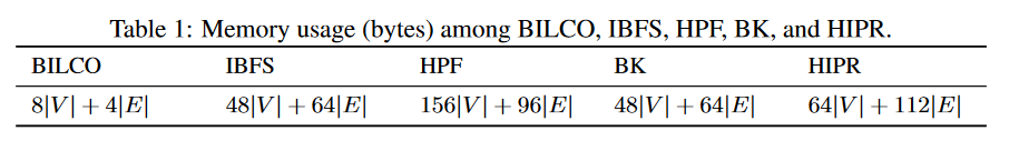
memory usage
BILCO also uses the structure of the GTW graph to improve memory efficiency. In a typical max-flow method, a large portion of memory is used to record the relationship between nodes and edges; in BILCO, since the graph structure is known, nodes and edges can be stored in coordinate order and the relationship can be derived from their positions. In real-world applications, the cost of storing components is not significant because the number of components is negligible compared to large |V| and |E|. Table 1 compares the memory usage of BILCO and peer methods based on their implementations.
experiment
Here we compare the efficiency of BILCO with four peer methods, IBFS, HPF, BK, and HIPR, under synthetic simulation and real applications. All experiments were performed in MATLAB using Intel(R) Xeon(R) Gold 6140@2.30Hz, 128GB memory, Windows 10 64-bit, and Microsoft VC++ compiler; no GPU was used; all experiments were performed in MATLAB. All methods were implemented in C/C++ using MATLAB wrappers.
composite data
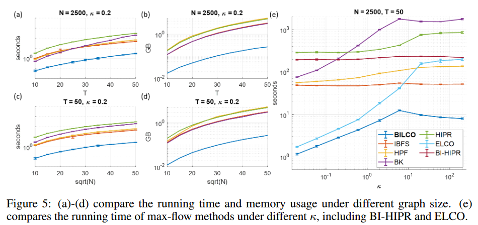
Simulated image signal propagation dataset with varying pixels (N ) and frames (T ), using a 4-connected neighbor, so the GTW graph is about |V | = 2N T 2 nodes and |E | = 7N T 2 edges. A bell-shaped signal propagates from the center of the image to the boundary. Gaussian noise was added to achieve a signal-to-noise ratio of 10 dB, mimicking a real-world scenario. To make the hyperparameters κ comparable, the synthetic data were normalized by dividing the standard deviation of the noise. 20 instances were tested for each combination of N, T, and κ.
Fig. 5(a-d) compares the BILCO and peer methods with different graph sizes, showing that the BILCO method is more than 10 times faster than any of the peer methods and requires only 1/10 of the memory cost. Fig. 5(e) shows the effect of the hyperparameter κ, comparing HIPR with the bi-directional pushing strategy (BI-HIPR) and the ELCO method. As can be seen, as the Ecross capacity increases, the execution time of most of the methods increases as κ increases because the degree of freedom of the exchange flow increases, and the graph becomes more complex as the Ecross capacity increases. Among all methods, BILCO shows the highest efficiency under any κ. Comparing ELCO and BILCO or HIPR and BI-HIPR, we see that the bidirectional pushing strategy speeds up both methods, especially under large κ. This is because the default initialization approaches the optimal solution as κ increases, effectively removing unnecessary computations. Fig. 5(e) also shows that the two strategies, ELCO and bidirectional push, are complementary and synergistic: when κ is small, ELCO dominates the acceleration; when κ is large, the bidirectional push has a greater impact; and when κ is small, ELCO has a greater impact. Interestingly, these two strategies synergistically increase speed when κ is large. For example, under the largest κ, both BI-HIPR and ELCO are nearly 4 times faster than HIPR, implying a 16-fold speedup of the independent effect, and BILCO is about 100 times faster than HIPR.
live data
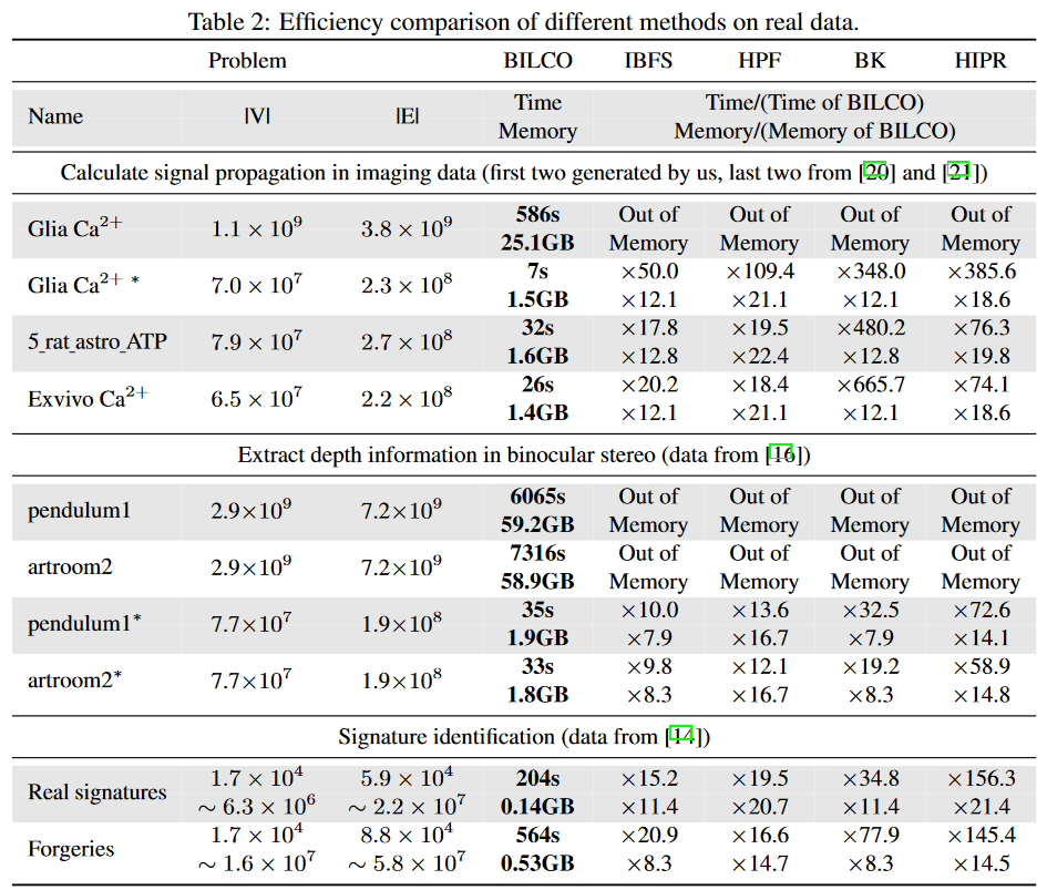
Here we compare our method BILCO with four peer methods in three different application categories: signal propagation computation, depth information extraction, and signature identification. Since all these max-flow methods give the same results, we compare only execution time and memory usage, as shown in Table 2. The * in the name represents spatially downsampled data, with BILCO as the baseline and how many times more costly the others are. The second application can derive depth from the misalignment of the same row between two images but assumes that the depth distributions of adjacent rows are similar. In this experiment, the window size is set to 1/5 of the array length to avoid unnecessary computations while allowing for relatively large disparities. The third application identifies 20 signatures and compares 500 authentic signatures and 500 forged signatures with a reference signature. The table shows the total execution time and maximum memory usage for the two signature categories. As can be seen, BILCO consistently performs best in all these joint alignment applications; BILCO shows a speedup of about 10 to 50 times compared to the best peer methods and requires almost 1/10th of the memory cost. In particular, for applications that estimate signal propagation, BILCO performs on average 29 times faster (in the 18 to 50 range) than other methods. Considering the diversity of these applications and the fact that the dependency structure varies from 2 adjacencies in the depth direction, to 4 adjacencies in the propagation direction, to all adjacencies in the signature direction, this is a powerful demonstration of BILCO's superiority and broad applicability.
Conclusion.
Compared to DTW, joint alignment exploits data dependencies to obtain better performance, but at the expense of speed and memory. In this paper, we exploit the peculiarities of this problem and develop the BILCO algorithm that minimizes these sacrifices. The algorithm can efficiently solve the joint alignment max-flow problem and obtain an exact globally optimal solution without sacrificing accuracy. In addition to theoretical analysis, we demonstrated the efficiency of BILCO through synthetic experiments and real-world applications, showing that BILCO is approximately 10-50 times faster and requires on average only 1/10th the memory cost compared to the best IBFS, HPF, BK, and HIPR methods. In addition, the results of validation under various scenarios suggest that BILCO applies to a wide range of applications. It is expected that this research will facilitate the application of joint alignment to achieve better performance in various fields.
The bidirectional push strategy can not only be viewed as a general push-label speedup technique but was found to work synergistically with BILCO's linear component operations. With the bidirectional push strategy, graphs are separated so there are fewer unwanted excesses and deficiencies, fewer saturated edges and cuts, and larger components. Since larger components significantly reduce the number of operations, BILCO is even faster (100×) than BI-HIPR (4×) and ELCO (4×) multiplications when compared to the aforementioned HIPR.
The BILCO algorithm is a special approach to certain max-flow problems. max-flow algorithms have a long history of invention, but existing methods, whether based on path extension, local operations like push relabel, combinations of both, or integration of graph decomposition but cannot solve the problem efficiently. To the best of our knowledge, this paper is the first to integrate DP and the general push-relabel method to solve the max-flow problem. There is a general feeling in this field that initialization is not very useful for max-flow algorithms, but here we have shown that bidirectional push is a good strategy to take advantage of initialization and is particularly powerful when combined with linear component operations. We hope that our efforts here will not only help in the application of joint alignment but also serve as a stimulus for developing methodologies for specific network flow problems. While it is difficult to invent better general-purpose algorithms for classical problems, they feel that there are many opportunities for more specific problems and that there is indeed a great demand for them due to the recent supersizing of problems.


Categories related to this article


