
Time Series Forecasting D3VAE Using Generative Models
3 main points
✔️ This is a NeurIPS 2022 accepted paper proposing a new method for time series forecasting using a generative model called D3VAE. It combines diffusion, denoising, and de-entanglement methods with a bi-directional variational autoencoder.
✔️ The goal is to address the problem of time series forecasting with limited and noisy data and to provide more stable and interpretable forecasts.
✔️ Extensive experiments on synthetic and real-world data are presented to demonstrate the effectiveness of the proposed method.
Generative Time Series Forecasting with Diffusion, Denoise, and Disentanglement
written by Yan Li, Xinjiang Lu, Yaqing Wang, Dejing Dou
(Submitted on 8 Jan 2023)
Comments: NeurIPS 2022 Accept
Subjects: Machine Learning (cs.LG)
code:

The images used in this article are from the paper, the introductory slides, or were created based on them.
summary
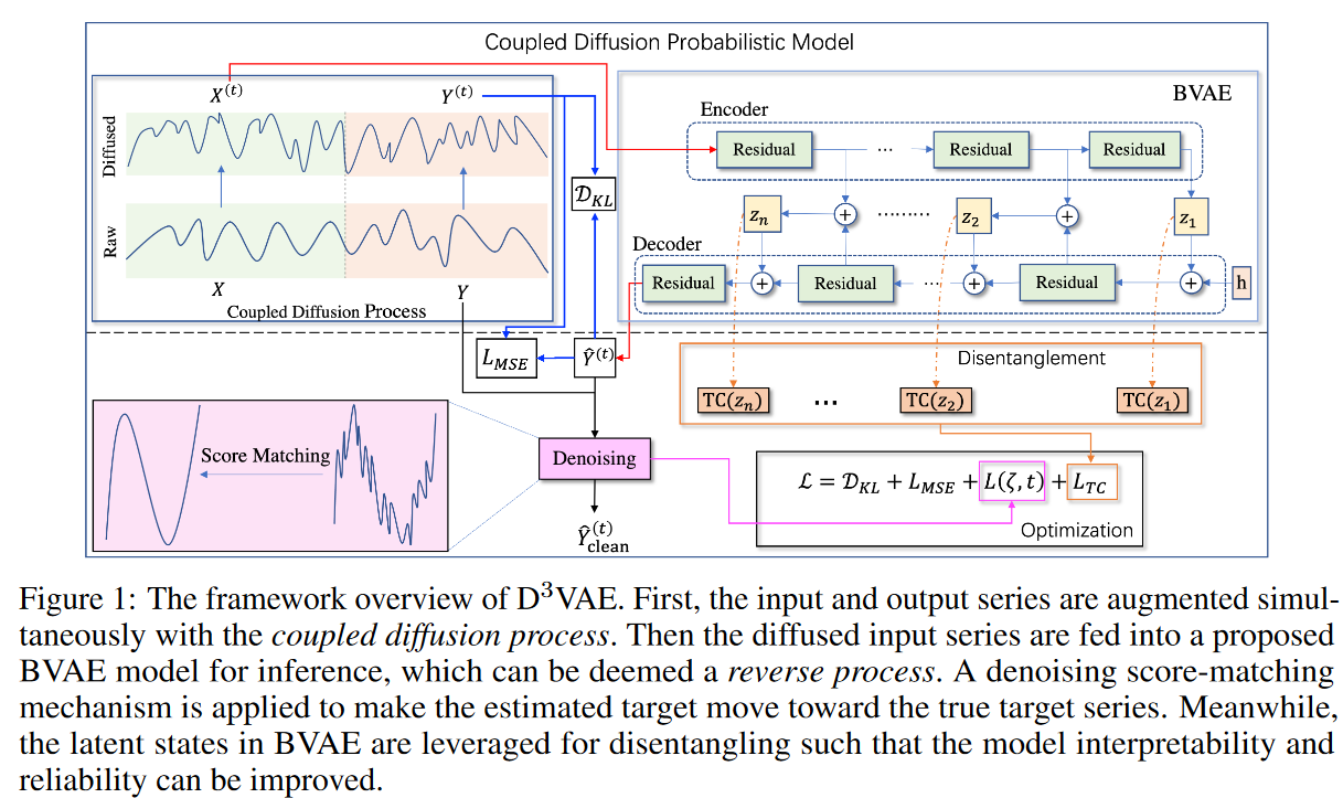
This is a NeurIPS 2022 accepted paper. The theme is time series forecasting. The paper proposes a new method of time series forecasting using generative modeling called D3VAE. The method combines diffusion, denoising, and de-entanglement methods with a bidirectional variational autoencoder (BVAE). The proposed method aims to address the problem of time series forecasting with limited and noisy data and to provide more stable and interpretable forecasts. Specifically, we propose a coupled diffusion probability model to augment time series data without increasing chance uncertainty and to implement a more tractable inference process in BVAE. Furthermore, we propose to adapt and integrate multiscale denoising score matching into the diffusion process for time series forecasting to ensure that the generated time series are truly goal-directed. Furthermore, to increase the interpretability and stability of the forecasts, we treat the latent variables multivariate and isolate them after minimizing their total correlations.
Introduction.
Time series forecasting is critical in risk aversion and decision-making. Traditional RNN-based methods predict the future by capturing the temporal dependence of time series. Long Short-Term Memory (LSTM) and Gated Recurrent Units (GRUs) effectively handle long-term dependence by introducing gated functions into the cell structure. Models based on convolutional neural networks (CNN) capture complex internal patterns of time series through convolutional operations. Recently, transformer-based models have shown excellent performance in time series prediction, demonstrating the ability of multi-headed self-attention. However, one of the major problems of neural networks in time series forecasting is uncertainty due to the properties of deep structures. Models based on vector autoregression (VAR), which attempt to model the distribution of time series from hidden states, can provide more confidence in forecasts, but their performance is not satisfactory.
Interpretable representation learning is another benefit of time series forecasting. Variational autoencoder (VAE) not only excels at modeling the latent distribution of the data and reducing gradient noise, but it also demonstrates the interpretability of time series forecasts. However, VAE may have poorer interpretability due to the latent variables involved.
Efforts are underway to learn representation dissimilarity, and it has been shown that a well-disentangled representation can improve the performance and robustness of the algorithm.
Furthermore, real-world time series are often noisy and recorded over short periods, which can lead to overfitting and generalization problems. For this reason, this paper addresses the time series prediction problem with generative modeling. Specifically, we propose a bidirectional variational autoencoder (BVAE) with diffusion, noise, and de-entanglement, or D3VAE. Specifically, we first propose a coupled diffusion stochastic model inspired by the forward process of diffusion models, which improves time series data limitations by augmenting the input and output time series. We also adapt Nouveau VAE to the time series forecasting task and develop BVAE as a proxy for the inverse process of the diffusion model. Thus, the expressive power of the diffusion model combined with the tractability of VAE can be used for generative time series forecasting. However, while it has the advantage of being generalizable, diffused samples can be corrupted, resulting in the generative model moving toward noisy targets. Therefore, in this paper, we further develop a scaled denoising score matching network to clean diffuse time series. We further isolate the latent variables in the time series by assuming that the different dimensions of the latent variables correspond to different temporal patterns (trends, seasonality, etc.).
The contributions here can be summarized as follows
- We propose a coupled diffusion stochastic model that aims to reduce the realistic uncertainty of time series and improve the generalizability of the generative model.
- We also integrate multiscale denoising score matching into the coupled diffusion process to improve the accuracy of the generative results.
- Latent variables in the generated model are separated to improve interpretability in time series forecasting.
- Extensive experiments on synthetic and real-world datasets demonstrate that D3VAE outperforms competing baselines by a satisfactory margin.
technique
Generation Time Series Prediction
Problem Formulation
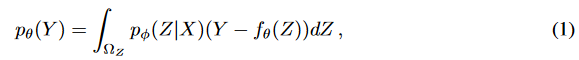
The input data is a multivariate time series X consisting of n data points, where each data point xi is a vector of dimension D. The corresponding target time series Y consists of m data points, and each data point yj is a vector of dimension d' (d' ≤ d). The goal is to generate the target time series Y from a latent variable Z extracted from a Gaussian distribution Z ~ p (Z|X). The distribution of the latent variable is formulated as pφ (Z|X) = gφ (X) where gφ is a nonlinear function. The data density of the target series is obtained by Equation (1). where pσ (Y) is the probability density function of the target series, fσ is the parameterization function, and Z is integrated over the latent variable space ΩZ. The target time series can be obtained by sampling from pθ (Y).
The time series prediction problem set here is to learn a representation Z that captures the useful signal of X and maps low-dimensional X to the latent space with high representativeness. an overview of the D3VAE framework is shown in Fig. 1. Before going into the detailed techniques, we first introduce some preliminary propositions.
Proposition 1
A time series X can be decomposed into Xr and X where Xr is the ideal noiseless time series data. The error between the ground truth and the prediction can be viewed as a combination of random and epistemic uncertainty.
Joint Diffusion Probability Model
Diffusion probability models (abbreviated as diffusion models) are a set of latent variable models aimed at generating high-quality samples. To make the generative time series forecasting model highly expressive, a coupled order process has been developed that synchronously augments the input and target series. In addition, more tractable and accurate forecasts are expected in the forecasting task. To this end, we propose a bidirectional variational autoencoder (BVAE) instead of the inverse of the diffusion model.
Coupled Diffusion Process
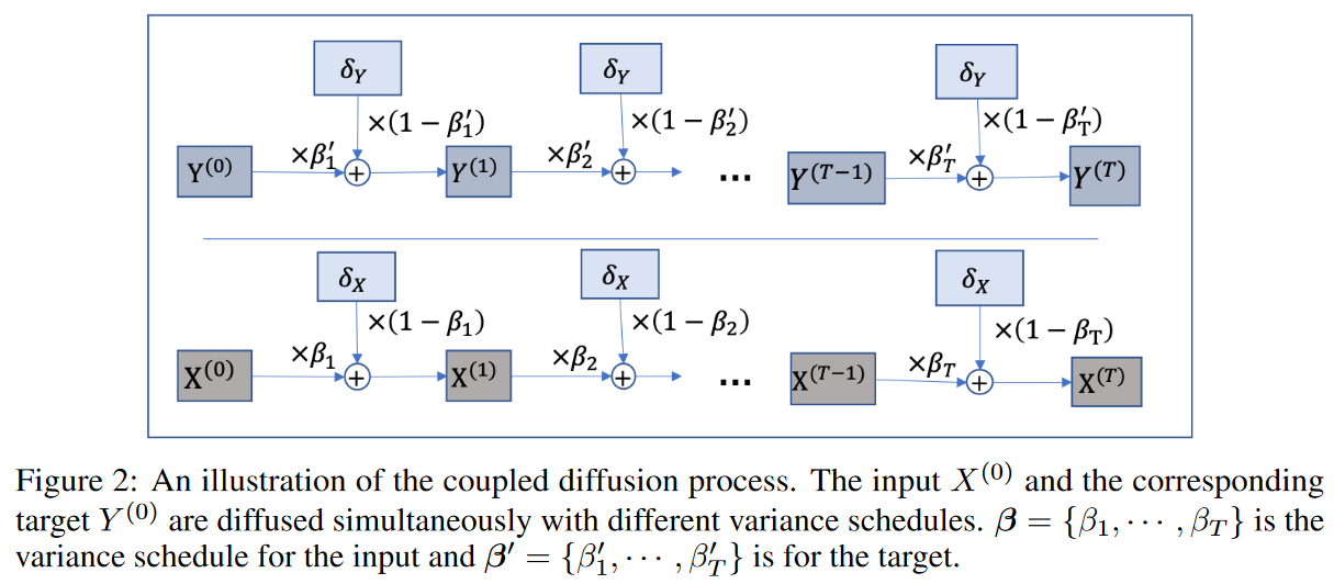
The forward diffusion process is anchored to a Markov chain that gradually adds Gaussian noise to the data. To diffuse the input and output sequences, we propose a coupled diffusion process as shown in Fig. 2. Specifically, given an input X = X(0) ∼ q(X(0)), the approximate posterior q(X(1:T )|X(0)) is obtained as follows

Here, a uniform increasing variance schedule β = {β1,-, βT | βt ∈ [0, 1]} is employed to control the level of noise to be added.Then, ifαt = 1 to βt, , we have

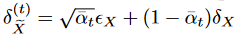
Furthermore, by Proposition 1, X(0) can be decomposed as X(0) = Xr, ϵX Then, using equation (3), we can decompose the diffused X(t) as follows

where δX denotes the standard Gaussian noise of X. Since α can be determined if the dispersion schedule β is known, the diffusion process also determines the ideal part. Now, if 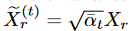 ,
,  , then by Proposition 1 and Equation (4), we have

Here, represents the noise generated by
 . To mitigate the effects of contingent uncertainty due to time series data, we further apply a diffusion process to the target series
 . Specifically, we adopt a scale parameter ω ∈ (0, 1) such that
 ,
, , and according to Proposition 1, we obtain the following decomposition (similar to Equation (4) )

As a result, q(Y (t)) = q( ̃ Y (t) r )q(δ(t) ̃ Y ). Proposition 1 and equations (5) and (6) can then be used to draw the following conclusions
For Lemma 1 ∀ε > 0, there exists a stochastic model fφ,θ:= (pφ, pθ) that guarantees  .Let
.Let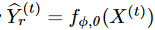 be the case here.
Lemma 2 The coupled diffusion process reduces the difference between diffuse and generated noise. Namely,
Thus, the uncertainty introduced by the generative model and data-specific noise can be reduced by the coupled diffusion process. Furthermore, the diffusion process simultaneously augments the input and target series, thus improving the generalization capability of (particularly short) time series forecasts.
Bidirectional Variable Auto Encoder
Traditionally, inverse processes are employed in diffusion models to generate high-quality samples. However, in generative time series forecasting problems, not only expressive power but also ground truth monitoring must be considered. In this study, we employ a more efficient generative model, namely the bidirectional variational autoencoder (BVAE), to perform the inverse process on behalf of the diffusion model. The architecture of BVAE is shown in Fig. 1, and
and where Z is treated multivariate. And n is determined by the number of residual blocks not only at the encoder but also at the decoder; another advantage of BVAE is that it opens an interface to integrate the discretization to improve the interpretability of the model.
Scaled Noise Removal Score Matching for Diffuse Time Series Cleaning
Although the time series data can be augmented with the coupled diffusion probability model described above, the generating distribution pθ( ̂ Y (t)) tends toward the corrupted diffusion target series Y (t). To further "clean" the generated target series, Denoising Score Matching (DSM) is employed to accelerate the uncertainty removal process without sacrificing model flexibility. DSM is a combination of Denoising Auto-Encoder (DAE ) and Score Matching (SM). Let ̂Y be the generated target series, the objective function is

where is the joint density of pairs of corrupt and clean samples ( ̂ Y, Y ),
 is the derivative of the log density of a single noise kernel, which is used to replace theParzen density estimator:
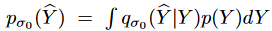 with score matching, and
  is the energy function. For the special case of Gaussian noise,
 , we therefore have

Then, for the diffuse target series at step t, we can obtain

To scale different levels of noise, a monotonically decreasing series of fixed σ values {σ1, - -, σT | σt = 1 - ̄αt} are employed. Thus, the objective function of the multiscaled DSM is

Let σ ∈ {σ1, - - - , σT } and l(σt) = σt. In equation (10), setting σ0 ensures that the gradient has the correct magnitude. In the generated time series forecasting setting, the generated samples will be tested without applying the diffusion process. To further denoise the generated target serieŝY, a single-step gradient denoising jump is applied:

The generated results tend to have a larger distribution space than the true target, and the noise term in equation (11) approximates the noise between the generated and "cleaned" target series. Thus,  can be treated as an estimated uncertainty in the forecast.
Isolating latent variables for interpretation
The interpretability of time series forecasting models is critical for many downstream tasks. Isolating potential variables in a generative model can further enhance not only interpretability but also the reliability of the forecast.
To isolate the latent variables Z = z1, ... zn, we attempt to minimize Total Correlation (TC), a standard metric for measuring the dependence between multiple random variables.

where m represents the number of factors in zi that need to be discretized. If the latent variableholdsuseful information, a lower TC generally means a better discretization. However, if the latent variable has no meaningful signal, we may get a very low TC. The bidirectional structure of BVAE allows us to deal with such problems without difficulty. as shown in Fig. 1, the signal is spread in both the encoder and the decoder, and rich semantics in the latent variable are aggregated. Furthermore, to mitigate the effect of latent irregular values, the sum of z1:n correlations can be averaged to obtain the loss to TC score for the BVAE:

Learning and Prediction
Training Objectives
To reduce the effects of uncertainty, we propose a coupled diffusion with a noise elimination network without sacrificing generality. We then isolate the latent variables in the generative model by minimizing the TC of the latent variables. Finally, we reconstruct the losses using several trade-off parameters. Using equations (10), (11), and (13), we obtain

where Lmse computes the mean squared error (MSE) between Y(t) and Y(t). By minimizing the above objective, the generative model is trained accordingly.
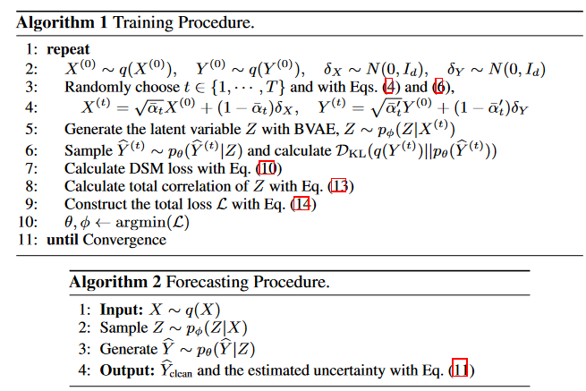
algorithm
Algorithm 1 shows the complete learning procedure for D3VAE using the loss function in Eq. (14). For inference, as described in Algorithm2, given an input series X, the target series can be generated directly from the distribution pθ, conditional on the latent state drawn from the distribution pφ.
experiment
setting (of a computer or file, etc.)
data-set
Generate two composite data sets.
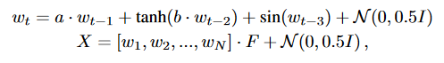
where wt R2 and 0 wt,1, wt,2 1 (t = 1, 2, 3), F R2×k [ 1, 1 ], k is the number of dimensions, N is the number of time points, and a and b are two constants. a = 0.9, b = 0.2, k = 20 for generatingD1, a = 0.5, b = 0.5, k = 40 for generating D2, and D1 and D2were set to N = 800 for both D1 and D2.
Six real-world datasets with diverse spatiotemporal dynamics were selected, including traffic, electricity weather, wind ( wind power ), and ETT(ETTm1 and ETTh1). To highlight the uncertainty of the short time series scenarios, for each dataset, we slice a subset from the starting point and ensure that each sliced dataset contains up to1000 time points:5%-Traffic, 3%-Electricity, 2%-Weather, 2%-Wind, 1%-ETTm1, and 5%-ETTh1.All datasets were split into time series and the same training/validation/testing ratiowasemployed, i.e. 7:1:2.
baseline
D3 VAE was compared to one GP (Gaussian process) based method (GP-copula), two autoregressive methods (DeepAR and TimeGrad), and four VAE-based methods (vanilla VAE, NVAE, factor-VAE (f-VAE for short and β-TCVAE )). The results are shown below.
Implementation Details
The input-lx -the predict-ly window is applied to roll the training set, validation set, and test set with a stride of one time step each, and this setting is adopted for all data sets. Below, the last dimension of the multivariate time series is selected as the target variable by default.
Adam optimizer is used and the initial learning rate is 5e-4. The batch size is set to 16 and learning to a maximum of 20 epochs, with early stopping. The number of entanglement release coefficients is chosen from {4, 8}, βt β is set in the range 0. 01 to 0.1, different diffusion steps T [100, 1000], and then ω is set to 0.1. The trade-off hyperparameters are set to ψ =0. 05, λ = 0.1, and γ = 0.001 for ETTand ψ = 0.5, λ = 1.0, and γ = 0.01 for the others.Continuous Ranked Probability Score (CRPS) and Mean Squared Error (MSE) are used as evaluation indices. For both evaluation indicators, the lower the better. In particular, CRPS is used to evaluate the similarity of two distributions and is equivalent to Mean Absolute Error (MAE) when the two distributions are discrete.
Main Results
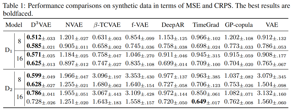
Two different predicted lengths were evaluated, i.e., ly 8, 16 (lx = ly ).
toy data set
Table 1 shows that D3 VAE achieves SOTA performance most of the time, while D2 achieves competitive CRPS at prediction length 16. Also, VAEoutperformsVAR and GP in D1, but VAR achieves better performance in D2, indicating the superiority of VAR in learning complex time dependencies.
Real-world datasets
In experiments on real-world data, D3VAE achieved consistent SOTA performance on the Wind dataset, except for forecast length 16 (Table 2). In particular, in the input-8-predict-8 setting, D3VAEwas able to produce significant improvements inMSEreductions (90%, 71%, 48%, 43%, 40%, 28%) for traffic, electricity, wind, ETTm1, ETTh1, and weather. for CRPS reductions, D3VAE was able to produce significant improvements in the input-8-predict-8 setting, traffic 73%, wind 31%, and electricity 27%; andinput-16-predict-16 setting, traffic 70%, electricity 18%, and weather 7% reductions.
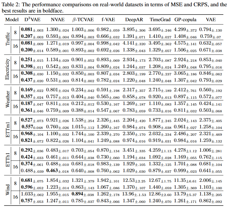
Overall, D3VAE has obtained, on average, a 43% MSE reduction and a 23% CRPS reduction in the above settings.
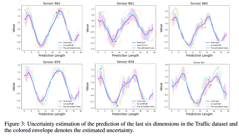
Uncertainty Estimation
Uncertainty can be evaluated by estimating the noise in the resulting series when making predictions. The scale parameter ω allows the generated distribution space to be adjusted accordingly.
The showcase in Fig. 3 demonstrates the uncertainty estimation of the generated series in the Traffic data set where the last six dimensions are treated as target variables. It can be seen that noise estimation can effectively quantify uncertainty. For example, when extreme values are encountered, the estimated uncertainty increases rapidly.
Entanglement Release Evaluation
In time series forecasting, it is difficult to manually label the separated factors, so take different dimensions of Z as the factors to be separated: zi = [zi,1, , zi,m ] (zi Z). The quality of separation can be evaluated by constructing a classifier that identifies whether instance zi,j belongs to class j or not and evaluating the classification performance. We also employ the mutual information content (MIG) as an indicator to evaluate entanglement release in a more parsimonious manner.
model analysis
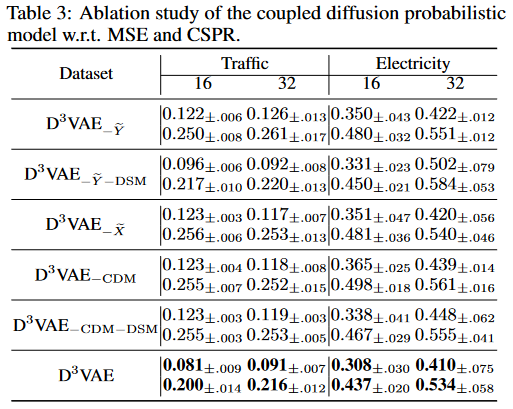
Ablation studies of coupled diffusion and denoising networks
To evaluate the effectiveness of the diffusion coupled model (CDM), the full version of D3VAE and its three variants
(i) D3VAE- ̃ Y, i.e., D3VAE without Y diffusion,
(ii) D3VAE- ̃ X, i.e., D3VAE without diffusing X,
(iii) D3VAE-CDM ( D3VAE without diffusion)
Comparisons will be made between the D3VAE We also report the performance of denoising score matching (DSM), denoted D3VAE-⑰ Y -DSM and D3VAE-CDM-DSM, when the target series is not diffuse. The truncation study is conducted on the Traffic and Electricity datasets under input-16-predict-16 and input-32-predict-32. the input or the target. We also see that if the target is not diffused, the denoising network is flawed because the noise level of the target cannot be estimated.
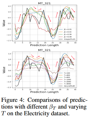
The dispersion schedule β and the number of diffusion steps T
To reduce the effects of uncertainty while maintaining an informative temporal pattern, the degree of diffusion must be appropriate. If the dispersion schedule is too small or the diffusion steps are insufficient, the diffusion process will be meaningless. Otherwise, the diffusion may become uncontrollable. Here we analyze the impact of the dispersion schedule β and the number of diffusion steps T. We set β1=0, vary the value of βt in the range [0.01, 0.1], and set T in the range 100 to 4000. as shown in Fig. 4, we can confirm that adopting appropriate β and T can improve the prediction performance.
discussion
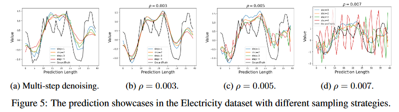
Sampling for Generated Time Series Forecasts
Langevin dynamics has been widely applied to energy-based model (EBM) sampling.

where k ∈ {0, - - -, K}, K is the number of sampling steps, and ρ is a constant; by setting K and ρ appropriately, high-quality samples can be generated. Langevin dynamics has been successfully applied in computer vision and natural language processing applications.
In this study, single-step gradient denoising jumps are employed to generate the target series. The experiments conducted demonstrate the effectiveness of such single-step sampling. Additional empirical studies will be conducted to investigate whether it is worth taking more sampling steps to further improve the performance of time series prediction; Fig. 5 shows the prediction results under different sampling strategies. To omit additive noise in Langevin dynamics, we employ D3VAE multistage denoising to generate the target series and plot the generated results in Fig. 5a. We then implement the generative procedure instead of denoising in standard Langevin dynamics and compare the generated target series with different ρ (see Fig. 5b-5d). We observe that in generative time series prediction, more sampling steps may not help improve prediction performance (Fig. 5a). Furthermore, more sampling steps are expected to be computationally expensive. On the other hand, different configurations of Langevin dynamics (varying ρ) do not provide essential benefits for time series forecasting (Figs. 5b-5d).
limit
Although the coupled diffusion probability model reduces the aleatoric uncertainty of the time series, it introduces a new bias in the time series to mimic the distribution of inputs and targets. However, due to the problem common to VAEs that bias in the inputs will also bias the outputs produced[, the diffusion step and dispersion schedule must be carefully chosen so that this model can be smoothly applied to different time series tasks. The proposed model is designed for general time series forecasting and should be used appropriately to avoid possible negative social consequences such as unauthorized applications.
In time series forecasting analysis, de-entangling latent variables is critical for interpreting more reliable forecasts. In generative time series forecasting, only unsupervised discretization learning is possible due to the lack of prior knowledge of entangled factors, and even though this has proven to be theoretically feasible for time series, for borderless applications of de-entanglement and better performance, it will be worth exploring how time series factors It is worth exploring how to label time series factors in the future for borderless applications and better performance. In addition, since time series data are unique, exploring more generative and sampling methods for the time series generation task is another promising direction.
summary
In this study, we propose a generative model with a two-way VAE as the backbone. For further generality, we devise a coupled diffusion probability model for time series forecasting. We then develop a scaled denoising network to guarantee prediction accuracy. We then further isolate potential variables to improve the interpretability of the model. Extensive experiments on synthetic and real-world data verified that the proposed generative model achieves SOTA performance compared to existing competitive generative models.


Categories related to this article


