
Contrastive Learning GraphTNC For Time Series On Dynamic Graphs
3 main points
✔️ GraphTNC proposes a novel encoder using a contrastive learning framework to learn the representation of multivariate time series data on dynamic or static graphs
✔️ The central architecture consists of a static The central architecture consists of a graph encoding module to learn the relationship between graph states and multivariate time series, and a temporal module to capture the dynamics of the data
✔️ Experimental results on synthetic and real datasets show that the method is effective when the graph informs and captures the dynamic relationships between signal features.
Contrastive Learning for Time Series on Dynamic Graphs
written by Yitian Zhang, Florence Regol, Antonios Valkanas, Mark Coates
(Submitted on 21 Sep 2022)
Comments: Published on arxiv.
Subjects: Machine Learning (cs.LG)
code:
The images used in this article are from the paper, the introductory slides, or were created based on them.
outline
In recent years, several attempts have been made to develop representations of multivariate time series in the framework of unsupervised learning. Such representations have proven beneficial in tasks such as activity recognition, health monitoring, and anomaly detection. In this paper, we consider a setting where we observe a time series at each node of a dynamic graph. We propose a framework called GraphTNC for unsupervised learning of a joint representation of graphs and time series. The approach uses a contrastive learning strategy. Assuming that the dynamics of change and evolution of the time series and graph are smooth in terms of segments, we identify local windows of time where the signal exhibits approximate stationarity. We then learn encodings that allow us to distinguish between the distributions of nearby and non-neighboring signals. We demonstrate the performance of synthetic data and a classification task on a real-world dataset.
first of all
Time series can be a challenging data type for modeling, especially supervised learning, due to their sparse labeling and complexity. To address this challenge, in this paper we use unsupervised methods to learn embeddings of time series, thereby extracting informative low-dimensional representations. Such a general representation of the input data does not require labels and can be used for any downstream task.
In the last few years, self-supervised learning (SSL) has been gaining attention as an effective method for representation learning.SSL is called contrastive learning and was popularized by "The simple framework for contrastive learning of visual representations", popularized by the SimCLR approach of "Simple framework for contrastive learning of visual representations". One of the dangers of self-supervised learning is decay due to the model outputting similar or identical embeddings for all samples. Contrastive learning avoids collapse by identifying positive and negative training pairs. The embeddings of samples in positive pairs are encouraged to be similar, while the embeddings of samples in negative pairs are pulled apart.
There are several approaches to contrastive learning of time series: Contrastive Predictive Coding (CPC) is an effective strategy that first compresses high-dimensional data into a compact potential embedding space and then uses autoregressive models to predict subsequent values of the signal. It uses the principles of predictive coding to train the encoder with stochastic contrast loss; Franceschi et al. in "Unsupervised scalable representation learning for multivariate time temporal Neighborhood Coding (TNC) use the local smoothness of the signal to learn a generalizable representation for a window of time series. This is achieved by ensuring that the distribution of signals close in time can be distinguished from the distribution far away in the representation space. TNC also considers the possibility that a pair of negative samples are also similar.
Uncontrolled learning is conceptually simpler than controlled learning and does not require large batch sizes or large memory banks to store negative samples. Notable approaches include Bootstrap Your Own Latent (BYOL) and Simple Siamese (SimSiam). These methods train the student network to predict the representation of the teacher network. The weights of the latter are either a moving average of the student weights or are shared with the students, but the gradient is not backpropagated through the teacher. Recent efforts have considered developing more effective loss terms. For example, Variance-Invariance-Covariance Regularization (VICReg ) is an improvement and construction of Barlow Twins loss, and Barlow Twins loss is an improvement and construction of EvoNet.
In some supervised learning frameworks, learning graph structures are considered to capture correlations in multivariate time series.
EvoNet can construct dynamic graphs from time series data and use them for event prediction. However, unsupervised representation learning of time series on graphs is still unexplored in the literature.
In this paper, we propose a framework called GraphTNC for learning a coupled representation of graphs and time series. The procedure is designed for settings where the underlying states of signals and graphs change over time. The model is scalable to time series with static graphs where the graph input at each time step is the same; we evaluate the quality of the representation trained on two datasets and show that the representation is general and transferable to downstream tasks such as classification. The contributions of this paper can be summarized as follows.
- We propose a new encoder using a contrastive learning framework to learn representations of multivariate time series data on dynamic or static graphs.
- We generalize non-contrastive learning methods from the computer vision field to non-stationary multivariate time series data.
problem-solving
We consider the task of unsupervised learning of the graphical representation of a time series. Let X ∈ RN× T be a multivariate time series, where N is the number of univariate time series and T is the total length of the time series. A window of fixed length w starting at time index t is contained by the [t, t + w]th column of X: X[t, t + w] ∈ RN×w and denoted Xt. w is not included in the notation as it is assumed constant and is specified only when necessary for clarity in the text. Associated with a multivariate time series is a dynamic graph with N nodes, whose edges evolve with the time series; each of the N univariate time series is associated with a single node in the graph. The edges between the nodes are assumed to represent the evolving correlation structure. Similar to the window of time series, we denote the window of the dynamic graph by Gt = [Gt, ..., Gt+w]; Gi = (V, Ei), |V| = N, where each graph Gi has associated with a graph state at the time i. The goal is to learn a representation zt∈Rh of a time series window and its associated graph (Xt, Gt):fenc(Xt, Gt)=zt.
technique
We design an architecture to build a representation of a multivariate time series window and its associated graph columns. This architecture is an encoder consisting of two modules. Below we describe these modules and the loss function used to train the encoder.
A. Encoder f enc ( Xt, Gt )
The encoding approach can be decomposed into two main building blocks a) A static graph encoding module to learn the relationship between graph states and multivariate time series b) A temporal module to capture the dynamics of the data
a) Static graph encoding module
The goal of this module is to learn the relationship between node embeddings and multivariate signals at time step i. To do so, we first need a representation of the individual nodes based on the states of the graph Gi. This is provided by an arbitrary node embedding function f G with the graph as input.
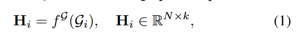
where k is the embedding dimension of the output node. We then concatenate the time series of this timestep, denoted by Hi and xi ∈ RN, and pass it through the neural network to obtain ei, the final representation of the interaction between the graph and the signal at timestep i.
![]()
where d is the dimension of the graph-signal interaction representation, vec(-) is the operator that stacks matrix columns, and [-|-] is the concatenation of two vectors (vec: Ra×b → Rab, [-||-]: Ra||Rb → Ra+b).
b) Temporal Module:
To capture the dynamic nature of the data (Xt, Gt ) and obtain the final representation zt, we use a time-based neural network f temp. This network f temp outputs the hidden state for the next time step si+1∈Rs based on the input of the current hidden state si∈Rs and time i. In this framework, the input is the signal xi coupled with the processed graph and the signal interaction ei. The final representation zt is obtained by passing the last hidden state of the window sw through the neural network: zt
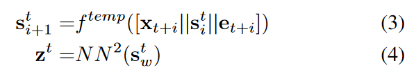
We use one-layer graph convolution as f G and one-layer bi-directional gated recurrent unit (GRU) as f temp. N N 1 and N N 2 are both one-layer feed-forward neural networks (FNN).
B. Loss Function
Define a discriminator D( zt, z). The objective function is to ensure that the probability likelihood estimate of the discriminator is close to 1 if z and zt are representations of a neighborhood window, and close to 0 otherwise. We consider a window that is close in time to be a neighborhood window and use the Augmented Dickey-Fuller (ADF) statistical test to find the neighborhood range. Since the underlying states of the graph and the signal are assumed to evolve together, the neighborhood Nt is chosen based on the time series only. The loss function is defined as
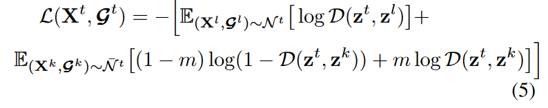
where m is the probability of sampling a positive window from a non-neighborhood ̄ N t. By optimizing the function, we can identify the representation zl = f enc (Xl, Gl) of samples from the neighborhood ( Xl,Gl ) ∈ N t with the representation zk = f enc ( Xk, Gk ) of samples from outside the neighborhood.
experiment
In our experiments, we evaluate the performance of the proposed model on a synthetic dataset in a controlled environment and on a real-world dataset. Both datasets have states that vary with time. Hence, a state is associated with each time window ( Xt, Gt). The performance of the trained representation z is evaluated by a downstream classification task where the states are the classification targets.
A. Dataset
1) Composite data
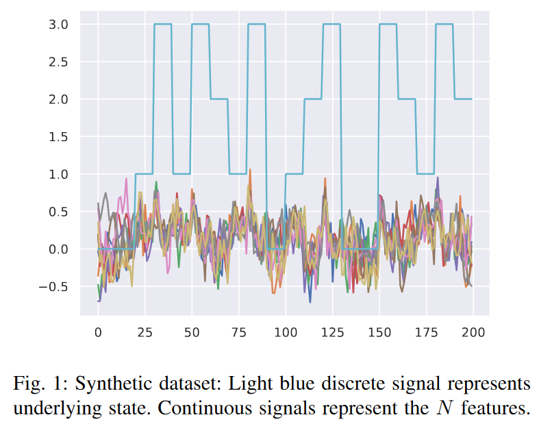
The synthetic dataset contains multivariate time series affected by the dynamic graph, which is also generated synthetically. The generation of the time series and graph is driven by the underlying state of the time series, which is modeled by a hidden Markov model (HMM). In each state, the time series are generated from different generative processes such as nonlinear autoregressive moving average models with different parameter sets or Gaussian processes with different kernel functions. The features of each time step are concatenated into a vector ft∈RN.
where At is the adjacency matrix of Gt and r is a weighted average of how much the graph affects the time series.
2) EEG: EEG signals are recorded from a probe connected to the subject's brain.
This dataset is from an online data science competition1 and contains 32-channel EEG recordings of subjects performing a hand grasping and lifting motion. Each hand movement is divided into seven states: initial movement, initial contact with the object being lifted, beginning of the loading phase, hand release, hand exchange, release, and no movement. The graphical structure of this dataset encodes the spatial relationships between the 32 electrode positions. This dataset provides a map of the physical location of the electrode probes relative to the brain. These probes are arranged in a grid. Each node represents an electrode probe, and if two probes are directly adjacent to the grid, an edge defines a graph connecting the two probes. Since the graph is static, it is repeated at each time step to fit this model; 100 signals of length 60-time steps are extracted to train the model.
B. Experimental setup
1) GraphTNC vs baseline TNC:
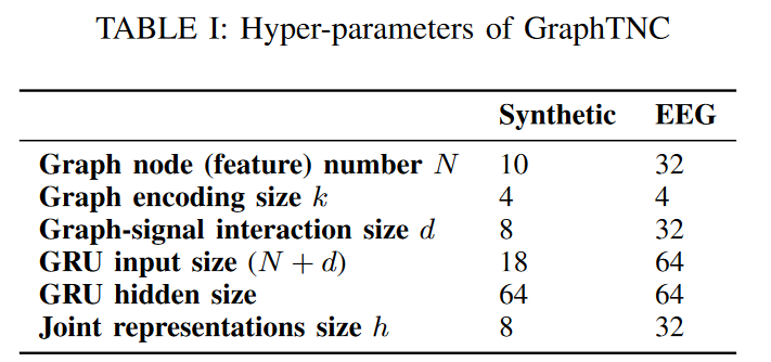
In this experiment, we compare the classification performance of representations learned from time series with and without considering the graph. To ensure a fair comparison, we use the same encoder proposed for the baseline TNC, f temp (a one-layer bi-directional GRU). In our architecture, we added a graph encoding module f G ( one-layer graph convolution) before the time module, so that the input of f temp is the synthetic information of the graph and the signal. See Table I for detailed hyperparameters.
We used the Adam optimizer for training, with a learning rate of 1e-3 and weight decay of 1e-5, 100 epochs, and early stopping for both datasets. As mentioned earlier, the discriminator and encoder are trained together during the training phase, but only the encoder is needed during inference. The window size w is chosen by experiment, based on the same theory as in TNC, to be long enough to contain the underlying state information, but not so long that it spans multiple states. To assess the quality of the representation, we use classification as a downstream task. The classifier is a one-layer FNN with h as the input dimension and S as the output dimension on top of the frozen representation and is trained with cross-entropy loss. By using a simple structure, the influence of the classifier on the final results is reduced: since AUPRC more accurately reflects the performance of the model on unbalanced data, the performance is reported as the prediction accuracy and the area under the precision-recall curve (AUPRC) score AUPRC is reported as predictive accuracy and area under the precision-recall curve (AUPRC) score.
2) Comparison of GraphTNC with uncontrolled learning
In this experiment, we retain the proposed encoder f enc ( Xt, Gt ) and compare the performance of the GraphTNC contrastive learning approach with two non-contrastive learning methods, BYOL and SimSiam. BYOL has a non-contrastive architecture and the weight θm of one encoder is the exponent of the other encoder's weight θ a moving average. The predictor g with weight φ is used in the branch with learnable weights; SimSiam uses a predictor in one branch and a stopping gradient operation in the other branch. In the original paper, the inputs to the two encoders are the original image and the reinforcement. To generalize these methods to the setting here, we feed (Xt, Gt ) and ( Xl, Gl ) ∈ Nt as positive pairs into the student-teacher network. Non-neighbor samples are not required; we use a two-layer FNN of size 128-128 for the projectors and predictors in both BYOL and SimSiam. We then compare the performance of all unsupervised approaches to a supervised model where the classifier and encoder are trained end-to-end. In the supervised setting, the encoder and classifier architecture is the same as in the unsupervised model. Here we evaluate the performance of representations learned from different methods by state classification accuracy and AUPRC.
C. Experimental Results and Discussion
1) GraphTNC vs. baseline TNC
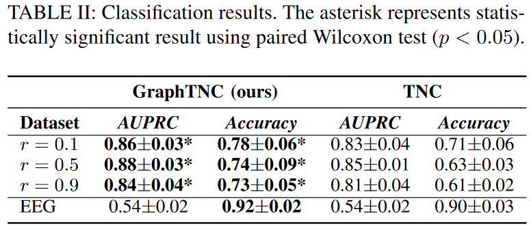
Table II shows the state classification results. The asterisk indicates that there is a statistically significant difference between GraphTNC and the baseline at the 5% level in the Wilcoxon signed-rank test. First, we observe that this encoder, which learns a combined representation of time series and graphs, consistently significantly outperforms the baseline most of the time, in the same parameterization order, for both simulated and EEG datasets. Therefore, we conclude that modeling the relationship between the features of the time series is expected to improve the performance.
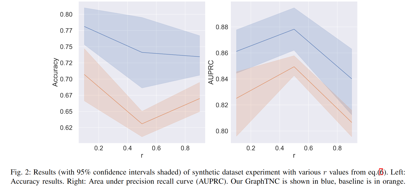
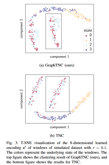
Next, to further understand how the role of the underlying graph affects performance, we generate multiple synthetic datasets with different values of the r parameter in Eq. (6). the larger r, the more dependent the time series data is on the graph-defined spatial filtering operation in Eq. (6) We conducted experiments for r ∈ {0.1, 0.5, 0.9}. We evaluate the model performance by training different models in 10 partitions for each r value and reporting their AUPRC. The proposed method GraphTNC (blue) consistently outperforms the time-series baseline TNC (orange). This is true for both the accuracy measure and the AUPRC. Given that the distribution of labels in synthetic data is not always uniform, it is essential to use both metrics; AUPRC is a combined precision and recall metric and is known to be a reliable metric for unbalanced data sets. In addition to reporting the mean and standard deviation of the results in Table II In addition to writing the mean and standard deviation of the results in Table II, we also report the 95% confidence intervals in Fig. 2. 95% confidence intervals are obtained by non-parametric methods (bootstrapping). We also present in Fig. 3 a visualization of the coding at r=0.1. It can be seen that the graph TNC representation is more clearly separated than the TNC representation, especially for the 0 and 2 states.
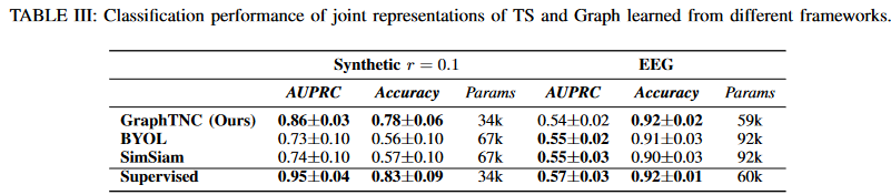
2) GraphTNC vs. uncontrolled learning
Table III shows the classification performance of the representations obtained from the different approaches on the two datasets, showing that the classification performance of GraphTNC is closer to the supervised model than the other two asymmetric learning methods. Also, the end-to-end learning framework has the same encoder as GraphTNC, followed by a single-layer FNN, so they have similar parameters. However, in the EEG dataset, BYOL and SimSiam can get reasonable results. However, when the non-stationarity increases, as in the synthetic data in Fig. 1, the performance degrades. Therefore, BYOL and SimSiam, which take nearby samples as reinforcement, are more suitable for more stable time series scenarios. On the other hand, these two non-contrastive learning methods require more parameters for training. In conclusion, GraphTNC proposed here is an effective approach for learning the representation of non-stationary time series on dynamic graphs.
summary
We introduce an unsupervised learning approach called GraphTNC for data consisting of multivariate time series on dynamic graphs. Experimental results on synthetic and real datasets show that the method is effective when the graph informs and captures the dynamic relationships between signal features.


Categories related to this article


