
Time Series Model LaST That Can Forecast Accurately Even With Mixed Seasonal Variations And Trends
3 main points
✔️ NeurIPS 2022 Accepted Paper. Proposes LaST, a forecasting model for time series data containing multiple fluctuating trends, including seasonal (periodic) fluctuations and trends
✔️ Separates multiple fluctuating trends and identifies each one using variational inference logic
✔️ Performance was tested using real-world data and found to be superior to seven previous models
Learning Latent Seasonal-Trend Representations for Time Series Forecasting
written by Zhiyuan Wang, Xovee Xu, Weifeng Zhang, Goce Trajcevski, Ting Zhong, Fan Zhou
(Submitted on 30 Dec 2022)
Comments: NeurIPS 2022
code:
The images used in this article are from the paper, the introductory slides, or were created based on them.
summary
This is a NeurIPS 2022 accepted paper. Recent attempts have been made to improve the prediction of time series by incorporating various deep learning techniques (RNN, Transformer, etc.) into sequential models. However, it is still difficult to extract clear patterns because time series are often composed of multiple, intertwined elements. Motivated by the success of computer vision and the separate-variate autoencoder in classical time series decomposition, this paper aims to infer some representations that describe the seasonal (periodic variation) and trend components of time series. To achieve this goal, we propose LaST, which is based on variational inference (variational Bayesian method) and aims to separate seasonality and trend representations in latent space. Moreover, LaST supervises and separates seasonality and trend representations in latent space, both in terms of themselves and in terms of input reconstruction, and introduces a set of auxiliary objectives. Extensive experiments prove that LaST achieves state-of-the-art performance on the time series forecasting task against state-of-the-art representation learning models and end-to-end forecasting models.
Note: For more information on variational Bayesian methods, see PRML (Pattern Recognition and Machine Learning) Chapter 10, etc.
Introduction
Due to the ubiquity and importance of time series data, a myriad of deep learning prediction models has recently been developed to improve time series prediction, attracting the efforts of researchers. these methods, based on advanced techniques such as RNNs and Transformers, typically learn a potential representation of each moment in a signal and then derive a prediction instrument to derive predictive results, achieving significant advances in the prediction task.
However, these models have difficulty extracting accurate and unambiguous information related to temporal patterns (e.g., seasonality, trends, levels), especially in supervised end-to-end architectures with no representation constraints. Efforts have therefore been made to apply variational inference to time series modeling, and improved guidance on latent representations with probabilistic forms has proven beneficial for downstream time series tasks. However, when there is complex co-evolution of various components in time series data, analysis with a single representation leads to superficial variables and a lack of model reusability and interpretability due to the high degree of entanglement of neural networks. Thus, while existing high-dimensional representation approaches provide efficiency and effectiveness, they sacrifice information utilization and explainability, and may even lead to overfitting and performance degradation.
To address the above limitations and explore a new disjunctive time series learning framework, this paper leverages the idea of a decomposition strategy to split time series data into several components, each capturing an underlying pattern category. Decomposition aids the analysis process and reveals fundamental insights that are more consistent with human intuition. Based on this insight, we took several latent representations corresponding to different time series characteristics (seasonality and trend in this case) and from there predicted the outcome by formulating the sequence as the sum of these characteristics. These latent representations should be as independent as possible to avoid models that have sufficient information on the input sequence but are prone to feature entanglement.
Therefore, in this paper we propose a new framework, LaST, to learn latent seasonality-trend representations for time series forecasting. laST utilizes an encoder-decoder architecture and follows variational inference theory to learn two discretized latent representations of time series seasonality and trend It learns. (1) From the input reconstruction, we isolate the unique seasonal and trend patterns that can be easily obtained from the raw time series and commercial measures and design a set of auxiliary targets accordingly. (2) From the representations themselves, minimize the mutual information (MI) between the seasonal/trend representations, under the assumption that consistency between the input data and each representation is guaranteed.
The three main contributions of this paper are
- Based on variational reasoning and information theory, we design a mechanism for learning and separating seasonality-trend representations and practically demonstrate its effectiveness and superiority over existing baselines in a time series forecasting task.
- We propose LaST, a potential seasonality-trend representation learning framework. It encodes the input as a separated seasonality-trend representation and provides a practical approach to reconstructing seasons and trends separately, avoiding chaos.
- We introduce the MI term as a penalty and present new tractable lower and upper bounds on its optimization. The lower bound ameliorates the problem of biased gradients in the traditional MINE approach and guarantees an information-rich representation. The upper bound provides feasibility to further reduce the overlap of the season-trend representation.
Framework for learning to represent potential seasonal trends
Although LaST uses seasonality and trend features to learn dissociation, this framework can be easily extended to adapt to situations where there are more than two components to be dissociated.
problem definition
Consider a time series data set D consisting of N i.i.d sequences denoted as x(i) 1:T = {x(i) 1, x(i) 2, - - -, x (i) t, - - -, x (i) T }, where i ∈ {1, 2, . .... } are univariate or multivariate values representing current observations (e.g., prices or rainfall) at time instant t, and each x (i) t is a univariate or multivariate value representing current observations (e.g., prices or rainfall) at time instant t. The goal is to derive a model that outputs a representation Z1:T suitable for predicting the future sequence Y = ˆ XT +1:T +τ. In the following, we omit superscripts and subscripts 1:T when there is no ambiguity. A model that infers the likelihood between an observation X and a future Y with a latent representation Z can be formulated as follows

In terms of variational inference, the likelihood P(X|Z) is calculated by the posterior distribution Qφ(Z|X) and is maximized by the following evidence lower bound (ELBO: evidence lower bound )
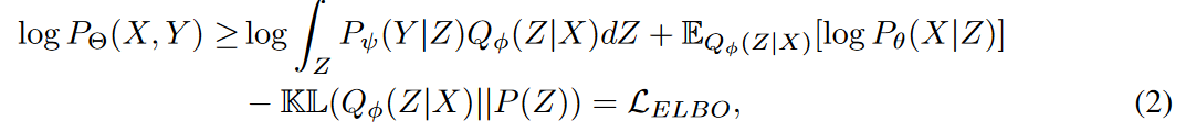
where Θ consists of ψ, φ, and θ and denotes the learned parameters.
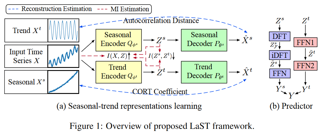
However, this runs into the problem of entanglement and cannot unambiguously extract complex temporal patterns. Therefore, to remedy this limitation, we incorporate a decomposition strategy into LaST to learn two separate representations for the dynamics of seasonality and trend. Specifically, we formulate the time signals X and Y as the sum of the seasonality and trend components, i.e., X = Xs + Xt. Thus, the latent representation Z is decomposed into Zs and Zt, assuming they are independent of each other, i.e., P (Z) = P (Zs)P (Zt) Fig. 1 shows two parts of the LaST framework: (a) representation learning to separate the seasonality-trend representation (separate reconstruction and MI constraints), and (b) forecasts based on the learned representations.
Theorem 1
With this decomposition strategy, equation (2) (i.e., ELBO) naturally takes the following factorized form
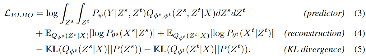
ELBO is divided into three main units, equations (3), (4), and (5). The predictor makes predictions and measures accuracy (e.g., L1 or L2 loss), while reconstruction and KL divergence are provided as regularization terms aimed at improving the learned representation. The three units are described below.
Predictor
This predictor variable can be considered the sum of two independent parts:![]() and
and ![]() . Here we present two specialized approaches to exploit the seasonality-trend representation, combining their respective characteristics. Given a seasonal latent representation Zs ∈ RT ×d, the seasonality predictor first uses a discrete Fourier transform (DFT) algorithm to detect the seasonality frequency. That is Zs F = DFT(Zs) ∈ CF ×d, where F = ⌊T +1 2⌋ is due to Nyquist's theorem. Next, we extend the representation back to the time domain with frequency to the future part, i.e., ̃ Zs = iDFT(Zs F ) ∈ Rτ ×d. Given Zt, the trend predictor provides a feedforward network (FFN) f: T → τ to generate a predictable representation ̃Zt∈Rτ×d ̃Zt ∈ Rτ×d. Map Zs and ̃ Zt to Y s and Y t, respectively, and terminate the predictor with two FFNs to obtain the predicted outcome Y by their sum.
. Here we present two specialized approaches to exploit the seasonality-trend representation, combining their respective characteristics. Given a seasonal latent representation Zs ∈ RT ×d, the seasonality predictor first uses a discrete Fourier transform (DFT) algorithm to detect the seasonality frequency. That is Zs F = DFT(Zs) ∈ CF ×d, where F = ⌊T +1 2⌋ is due to Nyquist's theorem. Next, we extend the representation back to the time domain with frequency to the future part, i.e., ̃ Zs = iDFT(Zs F ) ∈ Rτ ×d. Given Zt, the trend predictor provides a feedforward network (FFN) f: T → τ to generate a predictable representation ̃Zt∈Rτ×d ̃Zt ∈ Rτ×d. Map Zs and ̃ Zt to Y s and Y t, respectively, and terminate the predictor with two FFNs to obtain the predicted outcome Y by their sum.
Reconfiguration and KL divergence
Of these two terms, the KL divergence can be easily estimated by Monte Carlo sampling with prior assumptions. Here, for efficiency, we use the widely used setting where both prior distributions follow N (0, I). The reconstruction term cannot be measured directly, since Xs and Xt are unknown. Also, integrating these two terms into ![]() would make it easier for the decoder to reconstruct complex time series from any representation, leading to chaos.
would make it easier for the decoder to reconstruct complex time series from any representation, leading to chaos.
Theorem 2
Due to the assumption of a Gaussian distribution, the reconstruction loss Lrec can be estimated without utilizing Xs and Xt, and equation (4) can be replaced by the following equation
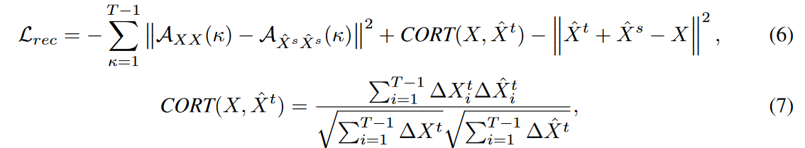
where![]() is the autocorrelation coefficient of the lagged value κ, CORT(X, ˆ Xt) is the time correlation coefficient, and ΔXi = Xi - Xi-1 is the first-order difference.
is the autocorrelation coefficient of the lagged value κ, CORT(X, ˆ Xt) is the time correlation coefficient, and ΔXi = Xi - Xi-1 is the first-order difference.
According to equation (6), reconstruction loss can be estimated and, conversely, can be used to supervise discretization representation learning. However, we found that this framework still has some shortcomings.
(1) KL divergence tends to reduce the distance between the posterior and the prior. It tends to sacrifice variational inference and data fitting when modeling capabilities are insufficient. In addition, the posterior estimate will have little information about the inputs and may result in predictions that are irrelevant to the observations.
(2) Seasonality - The non-connectedness of the trend expression is indirectly boosted by the separate reconstruction, where it is necessary to impose direct constraints on the expression itself.
By introducing an additional mutual information regularization term, we alleviate these constraints. Specifically, it increases the mutual information between Zs, Zt, and X, alleviates the divergence narrowing problem, and decreases the mutual information between Zs and Zt, further separating their representations.
LaST's maximization objectives are as follows
![]()
where I(-, -) represents the amount of mutual information between the two representations. However, these two mutual information terms are untraceable.
Mutual information bounds for optimization
We now address the traceable mutual information quantities that maximize I(X, Zs) and I(X, Zt) and minimize I(Zs, Zt) in equation (8) to show the lower and upper bounds of the model optimization.
Lower boundary of I(X, Zs) or I(X, Zt)
Among prior approaches to explore MI lower bounds, MINE, for example, uses the KL divergence between the joint distribution and the marginal to define an energy-based variational family to achieve a flexible and scalable lower bound. This can be formulated as  where γα can be the learning normalized clitic of the parameter α, but with a biased gradient due to the parametric logarithmic term. Replacing the logarithmic function with its tangent family improves the above-biased bounds.
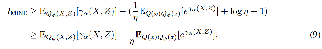
where η represents different tangents. The first inequality relies on a concave negative logarithmic function. The value on the curve is an upper bound on the value on the tangent and is tight when the contact point coincides with the true value of the independent variable, i.e. ![]() . The closer the distance between the tangent and the independent variable, the larger the lower bound. Therefore, let η be the variational term
. The closer the distance between the tangent and the independent variable, the larger the lower bound. Therefore, let η be the variational term![]() that estimates the independent variable to obtain as large a lower bound as possible. This inequality holds only when
that estimates the independent variable to obtain as large a lower bound as possible. This inequality holds only when![]() , meaning that γα can identify whether a pair of variables (X, Z) is sampled from the joint distribution or from the marginal. as with MINE, this consistency problem is addressed by the universal approximation theorem for neural networks The problem can be addressed by the universal approximation theorem for neural networks. Thus, Equation (9) provides a flexible and scalable lower bound for I(X, Z) with unbiased gradients.
, meaning that γα can identify whether a pair of variables (X, Z) is sampled from the joint distribution or from the marginal. as with MINE, this consistency problem is addressed by the universal approximation theorem for neural networks The problem can be addressed by the universal approximation theorem for neural networks. Thus, Equation (9) provides a flexible and scalable lower bound for I(X, Z) with unbiased gradients.
Upper boundary of I(Zs,Zt)
There has been little effort in the past to search for traceable upper bounds on the mutual information content. Existing upper bounds are traceable by joint or conditional distributions with known probabilistic densities (here Q(Zs | Zt), Q(Zt | Zs) or Q(Zs, Zt)). However, these distributions lack interpretability and are difficult to model directly, leading to untraceable estimates of the upper bound above.
To avoid directly estimating unknown stochastic densities, we introduce an energy-based variational family for Q(Zs, Zt) and set a traceable upper bound using a normalized clitic γβ(Zs, Zt) as in Equation (9). Specifically, the clitic γβ is incorporated into the upper bound ICLUB to obtain a traceable seasonality-trend upper bound (STUB) for I(Zs, Zt), which is defined as follows

The inequality in equation (10) is tight only if Zs and Zt are a pair of independent variables. This is precisely a sufficient condition for ISTUB, since both MI and equation (11) are zero in the independent situation, which is the seasonality-trend entanglement untangling the optimal objective. Critique γβ, like γα, has a discriminative role but provides an inverse score and constraints MI to a minimum. However, equation (11) can take negative values while learning the parameter β, resulting in an incorrect upper bound on MI. To alleviate this problem, we introduce an additional penalty term  to aid in model optimization, which is the L2 loss of the negative part of ISTUB.
experiment
Below, we present the results of an extensive experimental evaluation comparing LaST to the most recent baseline and present a series of empirical results, along with a visualization of the isolating study and seasonality-trend representation.
setting (of a computer or file, etc.)
Dataset and Baseline
Experiments were conducted on seven real-world benchmark datasets, each consisting of the following four categories of mainstream time series forecasting applications
(1) ETT. Electricity Transformer Temperature consists of the target "oil temperature" and six "power load" features, recorded hourly (i.e. ETTh1 and ETTh2) and every 15 minutes (i.e. ETTm1 and ETTm2) for two years.
(2) Electricity is preprocessed from the UCI Machine Learning Repository and contains hourly electricity consumption in kWh for 321 clients from 2012 to 2014.
(3) Exchange contains daily exchange rates for eight countries from 1990 to 2016.
(4) Weather includes 21 weather indicators (e.g., temperature and humidity) and is recorded every 10 minutes in 2020.
Compare LaST with state-of-the-art methods for two categories of time series modeling and forecasting tasks:
(1) Expression learning techniques including COST, TS2Vec, and TNC,
(2) End-to-end forecasting models such as VAE-GRU, Autoformer, Informer, TCN, etc.
Evaluation Settings
In previous studies, the model was run in both univariate and multivariate forecasting settings. In multivariate forecasting, LaST accepts and predicts all variables in the data set. In univariate forecasting, LaST considers only certain characteristics of each data set. For all datasets, standard normalization is employed and the input length T = 201. For the partitioning of the datasets, we follow the standard protocol of dividing the datasets into training, validation, and test sets in a time series with a ratio of 6:2:2 for all datasets.
Implementation Details
As for the network structure of LaST, we use a single-layer fully connected network as the feed-forward network (FFN), which is applied for modeling the posterior, reconstruction, and predictor. We also employed a two-layer MLP for the critic γ in MI boundary estimation. The dimensions of the seasonality and trend representations are matched. We set it to 32 for univariate forecasts and 128 for multivariate forecasts on other data sets.MAE loss is used to measure the predictions obtained from the predictor. The learning strategy uses the Adam optimizer and the learning process is stopped early within 10 epochs. The learning rate is initialized at 10-3 and decays with a weight of 0.95 per epoch.
Performance Comparison and Model Analysis
Effects
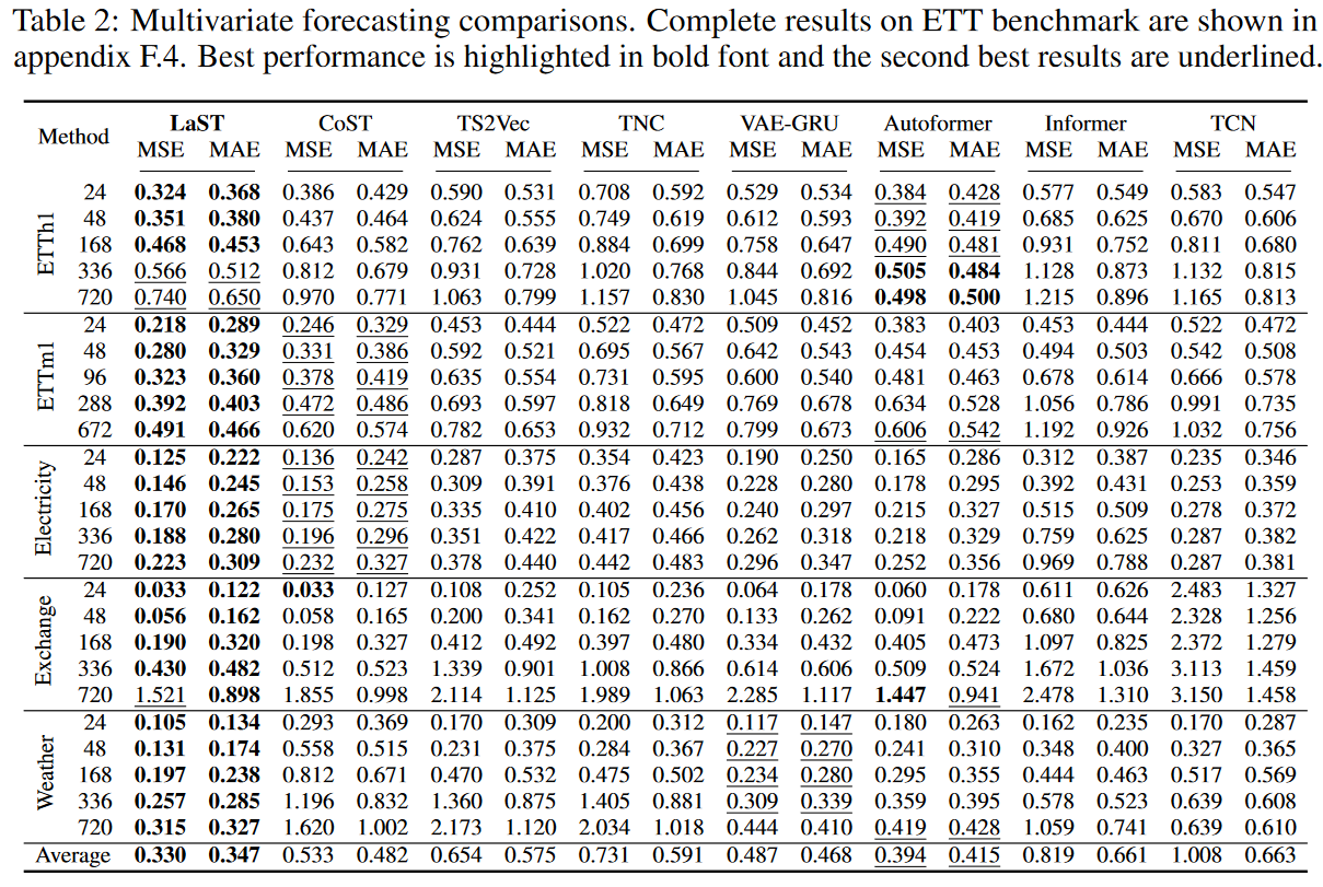
Table 1 and Table 2 summarize the results for univariate and multivariate forecasts, respectively. LaST achieves state-of-the-art performance against advanced representation baselines on five real-world datasets. the relative gains for MSE and MAE are 25.6% and 22.1% for the best representation learning method CoST and 22.0% and 18.9% for the best end-to-end model Autoformer. We note that Autoformer achieves better performance on long-term forecasts for the hourly ETT dataset, and we believe there are two reasons for this:
(1) Transformer-based models inherently establish long-range dependence, which plays an important role in long-term sequence prediction
(2) We employ a simple decomposition by mean pooling with a fixed kernel size, which is more appropriate for a highly periodic data set of hourly ETTs.
While this phenomenon is beneficial for long-term forecasting, its sensitivity to local context is limited, and the bonus does not have a significant impact on other data sets. Compared to baselines, LaST adaptively extracts patterns of seasonality and trends in a dissociated representation, making it applicable to intricate time series.

Resolution
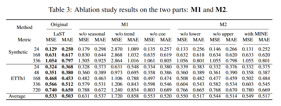
We investigated the performance benefits of each of the LaST mechanisms on the synthetic dataset and on ETTh1. The results are shown in Table 3 and consist of two groups: M1 examines the mechanisms of the seasonality-trend representation learning framework. In it, "w/o seasonal" and "w/o trend" represent LaST without the seasonal and trend components, respectively, and "w/o coe" represents LaST without the autocorrelation and CORT coefficients when estimating reconstruction losses. m2 judges the introduction and estimation of MI and uses "w/o lower " and "w/o upper" to represent the removal of the lower and upper limits of MI in the regularization term, respectively, and "with MINE" represents the replacement of the lower limit with MINE. The results show that all mechanisms improve the performance of the forecasting task. When the trend component is removed, we find a significant decrease in quality. The reason for this is that seasonal forecasting is derived from the iDFT algorithm, which is essentially a periodic repetition of past observations. However, capturing seasonal patterns and assisting the trend component with full LaST can provide an advantage, especially in long-term settings and strongly periodic synthetic data sets. Furthermore, when using the biased regularization term MINE, performance becomes unstable, sometimes worse than LaST without the MI lower bound, but the unbiased lower bound (see equation (9)) is found to continuously outperform LaST.
Expression Unwinding
Fig. 2 visualizes the representation of seasonal trends using the tSNE methodology. We also visualized the embedding in the final layer of the Autoformer decoder as a comparison. We can see that the same colored dots are mixed for no decomposition mechanism ("w/o dec" indicates the removal of two decomposition mechanisms (autocorrelation and CORT coefficients, as well as upper MI limits), whereas they are more clearly and tightly clustered for LaST.
It is also noteworthy that Autofomer with simple moving average blocks achieves a satisfactory decomposition in terms of time series, but its representation is still tangled. These results suggest that (1) it is not easy to learn to separate seasonality-trend representations, and (2) the proposed decomposition mechanism is successful in separating seasonality-trend representations in latent space, focusing on specific temporal patterns.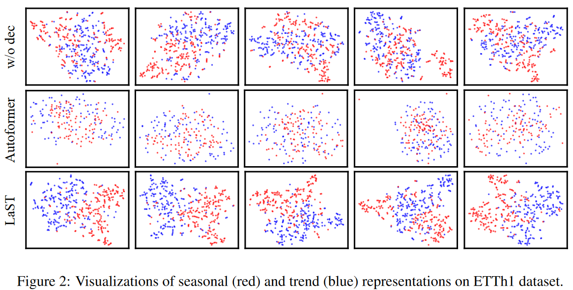
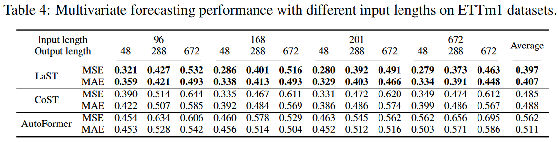
Input setting
To further validate the sensitivity, we examined the effect of hyperparameter input length, and Table 4 shows the results. Long lookback windows improve performance, especially for long-term forecasts, while others even degrade performance. This validates that LaST can effectively use historical information to understand patterns and make forecasts.
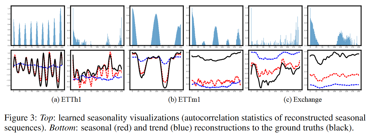
From the case studies
We further validated LaST by visualizing the extracted seasonality and trends with specific examples; as shown in Fig. 3, LaST can capture seasonal patterns in real-world data sets. For example, the hourly and 15-minute ETT data sets show strong intraday cycles; despite the lack of clear cycles in the Exchange data set, LaST provides several long-term cycles in the daily data. Furthermore, the trend and seasonal components accurately reconstruct the original series in terms of each, confirming LaST's ability to generate viable, separated representations for complex time series.
previous work
Most deep learning methods for time series prediction are designed as end-to-end architectures. Various basic techniques (e.g., residual structures, autoregressive networks, convolution ) are used to generate expressive nonlinear hidden states and embeddings that reflect time dependencies and patterns. There is also a group of studies applying Transformer structures to time series prediction tasks, which aim to discover relationships across sequences and focus on critical time points. Deep learning methods have achieved superior performance compared to classical algorithms such as ARIMA and VAR, and are popular in multiple applications.
Learning flexible representations has been demonstrated by several studies to be beneficial for downstream tasks. In the time series representation domain, early methods using variational reasoning jointly learn an approximate latent representation by learning an encoder that reconstructs the raw signal and its corresponding decoder. Recent efforts have improved these variational methods by using techniques such as copulas and normalized flows to establish more complex and flexible distributions. Another group uses burgeoning contrast learning to obtain invariant representations from extended time series, which avoids the reconstruction process and improves the representation without additional supervision.
Time series decomposition is a classical method of partitioning a complex time series into several components to obtain temporal patterns and interpretability. Recent research has applied machine learning and deep learning approaches to achieve robust and efficient decomposition for large data sets. There are also research efforts that address forecasting with the aid of decomposition. For example, Autoformer decomposes time series into seasonality and trend portions through mean pooling and introduces an autocorrelation mechanism to enhance Transformer for better relationship discovery; CoST encodes signals into seasonality and trend representations in the frequency and time domain, respectively, and introduces contrast learning to supervise their learning. These methods differ from this paper in that they utilize a simple mean pooling decomposition mechanism, which provides incompatible periodic assumptions and intuitively isolates representations by processing them in different domains. LaST, on the other hand, facilitates separation from a probabilistic perspective by adaptively extracting seasonality and trends of the separated representations in the latent space.
summary
This paper described LaST, a separate variational inference framework with mutual information constraints for separating mixed seasonality-trend representations in latent space for effective prediction of time series. Extensive experiments have demonstrated that LaST successfully separates seasonality-trend representations and achieves state-of-the-art performance. In the future, they will focus on tackling other challenging tasks downstream of time series, such as time series generation and assignment interpolation. In addition, they plan to explicitly model stochastic factors in their decomposition strategy to better understand real-world time series.


Categories related to this article


