
Time Series Imputation Network STING Based On Self-Attention Using GAN
3 main points
✔️ Propose a new imputation method for multivariate time-series data called STING (Self-attention based Time-series Imputation Networks using GAN )
✔️ Introduces a novel attention mechanism to avoid potential bi as
✔️ Outperforms existing state-of-the-art methods in terms of replacement accuracy and downstream tasks using replaced values
STING: Self-attention based Time-series Imputation Networks using GAN
written by Eunkyu Oh, Taehun Kim, Yunhu Ji, Sushil Khyalia
(Submitted on 22 Sep 2022)
Comments: Published on arxiv.
Subjects: Machine Learning (cs.LG); Artificial Intelligence (cs.AI)
code:
The images used in this article are from the paper, the introductory slides, or were created based on them.
outline
One of the most common problems with time series data used in many real-world applications is that time series data can have missing values due to the inherent nature of the data collection process. Therefore, imputing missing values from multivariate (correlated) time series data is essential for improving predictive performance while making accurate data-driven decisions. Traditional imputation only removes missing values or fills in missing values based on averages or zeros. In recent years, methods based on deep neural networks have attracted much attention, but they are still limited in capturing the complex generative process of multivariate time series. In this paper, we propose a novel imputation method for multivariate time-series data called STING (Self-attention-based Time-series Imputation Networks using GAN). It utilizes a generative adversarial network and a two-way recurrent neural network to learn a latent representation of the time series. In addition, we introduce a novel attentional mechanism to capture weighted correlations across time series and avoid potential biases introduced by irrelevant correlations. experimental results on three real-world datasets show that STING outperforms existing state-of-the-art methods in terms of replacement accuracy and downstream tasks using replaced values. the point, showing that STING outperforms the existing state-of-the-art methods in terms of
first of all
Many real-time application areas of multivariate time series data analyze these signals and perform predictive analysis. For example, financial marketing on stock price prediction, patient medical diagnosis prediction, weather forecasting, and real-time traffic forecasting. However, time series data inevitably contain missing values for some reason, such as certain data features being collected later or records being lost due to equipment damage or communication errors. In the medical field, for example, certain information collected from biopsies can be difficult or even dangerous to obtain. These types of missing data can severely degrade the quality of the model and even lead to wrong decisions by introducing a significant amount of bias. Therefore, embedding missing values in time series is of paramount importance for accurate data-driven decision-making.
Traditional missing-value assignment methods can be classified into two categories: discriminative and generative. The former includes Multivariate Imputation by Chained Equations (MICE) and MissForest, while the latter includes algorithms based on deep neural networks, such as Denoising Auto Encoder (DAE) and Generative Adversarial Networks (GAN)). However, these methods have been developed for non-time-series data, and thus may have little consideration of the temporal dependence between observations in a time series. In particular, DAE requires complete data during the training phase, a requirement that is almost impossible to meet because missing values are part of the intrinsic structure of the problem. Recent work for time series data imputation is based on recurrent neural networks (RNNs) and GANs. These capture various aspects and time dependencies of the observed (or missing) data properties, such as temporal decay, feature correlation, and temporal belief gates.
Here we propose a novel imputation method for multivariate time-series data, STING (Self-attention-based Time-series Imputation Network using GAN). The basic architecture of STING is a generative adversarial network that can estimate the true data distribution when imputing incomplete time-series data. Specifically, the generator learns the underlying distribution of multivariate time series data to accurately impute missing values, and the discriminator learns to distinguish between observed and imputed elements. To learn potential relationships between observed values with non-fixed time lags, the generator in GAN uses a new RNN cell GRUI (GRU for Imputation) internally to learn potential relationships between observations with non-fixed time lags. We weigh the impact on past observations according to the time lag. To impute the current missing values using information from both future and past observations, we employ a bi-directional RNN (B-RNN) to estimate variables from both forward and backward directions. Furthermore, we propose a novel attention mechanism that selectively focuses on relevant information in each time series. Experimental results on three real-world datasets show that STING outperforms state-of-the-art methods in terms of imputation performance. The model also outperforms the baseline on the post-imputation task, an indirect measure of replacement performance.
related research
Che et al. proposed a Gated Recurrent Unit with Decay (GRU-D), which learns missing patterns in incomplete time series and predicts target labels while filling in missing values in a healthcare dataset. The model uses RNNs and considers a weighted combination of its last observation and the empirical mean. They introduced an input decay rate and a hidden state decay rate to control the decay coefficient. However, this model makes the basic assumption that missing patterns in the data are often correlated with the target label (i.e., informative missing). Taking this fact into account, we take a unified approach by integrating the imputation and prediction tasks (i.e., of target labels) into a single process. This makes the model less general, as it relies on the target label being fully observed. This makes it difficult to use in an unlabeled unsupervised setting or when the labels are not clear. We also impose the statistical assumption that the inferred value is the ratio of the last observation to the empirical mean.
In a similar work, Cao et al. proposed an RNN-based method called BRITS (Bidirectional Recurrent Imputation for Time Series), which directly learns missing values that are considered latent variables in a bidirectional RNN graph. It combines history-based and feature-based estimation for feature correlation and applies a learning strategy that allows the missing values to take on a delayed gradient. However, the goal is to learn the imputation as well as to predict the target label based on the given time series. Therefore, we need to know the target label in the learning phase. However, this is a rather strong constraint since the target labels may be unknown or contain missing values. As a result, the performance of Imitation is very sensitive to the completeness of the target labels. Unlike them, the model in this paper does not depend on the target label in any process.
Luo et al. proposed a GAN-based imputation model called GAN-2-stages. To model distributions with temporal irregularities, they proposed a Gated Recurrent Unit for Imputation (GRUI), which learns to attenuate the effect of past observations according to the length of time-lapse in irregular time intervals. They further learn the input "noise" of the generator and find the optimal noise from the potential input space so that the generated sample is most similar to the original sample. However, whereas the original sample has a different time decay depending on the degree of missingness, the generated sample has the same time decay depending on completeness. This distinct difference in time decay allows the discriminator to better distinguish between false data and real data, which leads to faster discriminator convergence and prevents stable training of the generator. Furthermore, it is a self-feeding learning method, where incorrect outputs during training continue to be reflected in subsequent training until the end of the training process.
Luo et al. propose an End-to-End Generative Adversarial Network (E2GAN). They use a compression and reconstruction strategy that avoids the "noise" optimization stage with a denoising autoencoder. In the generator, random noise is added to the original time series as input and the encoder attempts to map the input to a low-dimensional vector. The decoder then reconstructs it from the low-dimensional vector and generates samples. Through this process, E2GAN was able to force a compressed representation of the input while learning the distribution of the original time series. However, E2GAN still suffers from the limitations of the GAN-2-stage, such as the fast convergence of the discriminator compared to the generators and RNN self-learning. In this paper, we employ a bi-directional delayed gradient to quickly and efficiently train RNN models in the generator using observations. Moreover, the proposed discriminator tries to solve a more specific problem by identifying whether each element of the input matrix is true (observed values) or false (generated values), rather than the entire input matrix, thus enabling stable adversarial learning.
problem description
Let the multivariate time series data X = {x1, x2, ..., xT } be a sequence of T observed values, and the t-th observed value xt ∈ RD consists of D features {xt1, xt2, . , xtD}. That is, xtd is denoted as the value of the d-th variable in xt. X is an incomplete matrix with missing values. We also introduce a mask vector mtd to indicate the position of the missing variable in xt. So, mtd is defined as follows
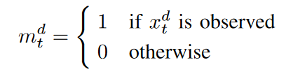
If xtd is a missing value, define X hat is approximately the same as X except that it is 0. Since time stamp time intervals are not always the same, we define δd t to be the time interval between the last observation and the current time stamp st.
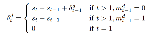
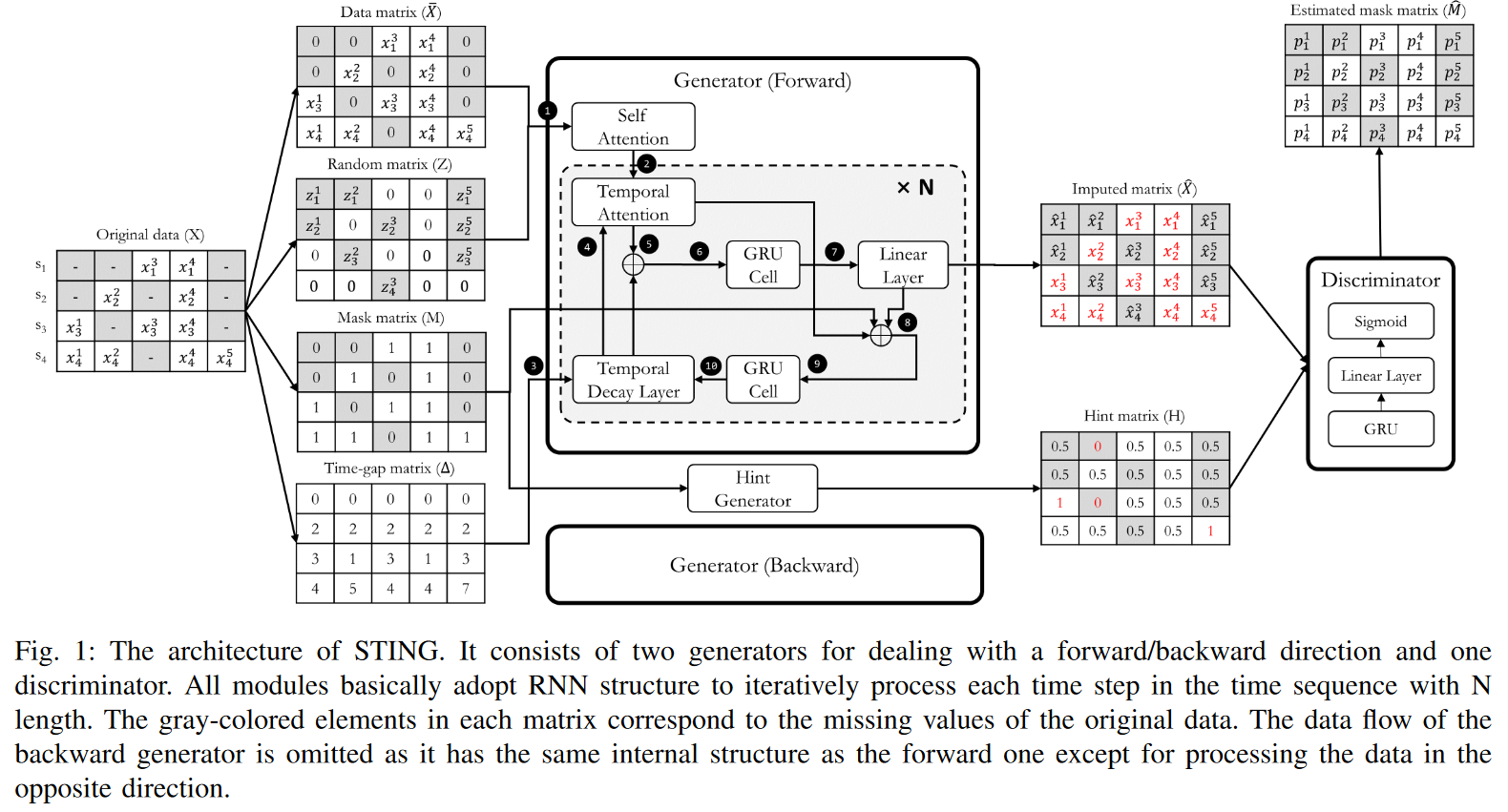
An example with input matrices is shown in Fig. 1. In this example, S is defined as S = {0, 2, 3, 7, sT }.
The goal is to accurately impute the missing values of the incomplete matrix X by the adversarial learning mechanism of the GAN. The generator tries to learn the underlying distribution of X to produce a complete time series matrix ˆ X, and the discriminator tries to match the estimated mask matrix ˆ M with the mask matrix M by identifying whether each element of the complete matrix is a real value from X or a false value from ˆ X. Each element of ˆ M represents the probability that each element of ˆ X is real-valued. We denote this probability as pdt ∈ [0, 1].
technique
In this section, we describe how to build an imputation model for multivariate time series data, focusing on the architecture and overall workflow shown in Fig. 1.
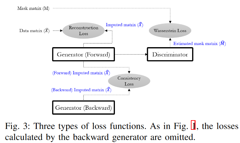
Inspired by existing deep generative neural networks, STING consists of two generators (Gs) and one discriminator (D); the two Gs take forward and inverse time series as input and each generates a time series matrix ˆ X according to a specified direction. The generation in both directions complements the problem of missing information in the unidirectional GRU structure, which suffers from a large number of missing values in the time series data. The interior of G consists of two attention modules and two modified GRU cells. The attention module computes correlation weights for the entire sequence, which can provide many clues to subsequent GRU modules. And the two GRU cells are designed to deal with time series inputs with irregular time intervals. On the other hand, D has a relatively simple structure compared to G, consisting of a GRU module for time series processing, a linear layer for dimensionality reduction, and finally a sigmoid activation that produces the probability of each element as an output.
From a workflow perspective, our approach begins by filling ̄ X with zeros for each missing value and then replacing those elements with zd t. M serves to inform G which elements of X are observed or missing values. This allows G to determine which values of the previous timestamp are reliable or unreliable when generating ˆ xt repeatedly. ∆ Also, ∆ has important information about how much previous hidden state G should refer to when there are arbitrarily missing values. Based on these four input matrices, G generates an imputation matrix ˆ X and refines it by filling in the observed values of X, since it does not need to generate xtd, which it already knows. That is, ˆ xtd is replaced by xtd if its elements are observables. This is the result of the imputation and is forwarded to the discriminator.
On the other hand, D takes ˆ X as input and learns to distinguish whether each element is an observed value or not. In this case, the hint matrix H is also given as an additional input, informing D about certain parts of M and directing its attention to specific components; H reveals some parts of M with htd = 0 (as missing values) or htd = 1 (as observed values). Furthermore, htd = 0.5 suggests nothing about the mtd that D's learning could be focused on. This is because D has to choose between 0 and 1 for a sample point of 0.5, which is a relatively difficult learning point, and D will concentrate on getting a better fit. In other words, without the hint mechanism, G is not guaranteed to learn the desired distribution that is uniquely defined by the original data. The amount of hint information about M can be controlled by varying H in the hint generator. The more hints, the easier D is to learn. Finally, the output of D is ˆ M, where each element represents the probability pdt that each element of ˆ X is an observed value.
By jointly training G and D via the min-max game, G learns the underlying distribution of the original data X and can properly impute missing values so that D cannot distinguish them; the ideal outcome for G is that each ptd of ˆ M corresponding to a generated false value ˆ and is set to 1. Thus, the ideal outcome of D is that each ptd corresponding to a false value ˆ xtd is set to 0, otherwise, it is set to 1. This means that D correctly predicts the result ˆ M equal to the mask matrix M. One feature of STING is that D attempts to distinguish which elements of the matrix are real (observed values) or false (attributed values), rather than the entire input matrix. This strategy allows D to focus more on specific classification problems, thereby improving performance.
A. Generator
STING utilizes two types of generators (i.e., forward G and backward G) to account for dependence in both directions in time, as shown in Fig. 1. The roles of both generators are the same, except for some of them, which will be discussed in the "Consistency Loss" section below. Therefore, for the majority of this section, we will only discuss the details of forward Gs and omit the description of backward Gs due to space limitations. Each G consists of a sophisticated GRU structure with two types of attention layers (self-attention and temporal attention), a temporal decay layer, and a double GRU cell. The detailed structure and learning objectives are as follows.
Attention aims to learn structural dependencies between different coordinates of input data by finding the most relevant parts of the input given a query value and generating a query-responsive representation. Attention mechanisms are effective in a variety of areas by learning the structural properties of the underlying data distribution. For example, in machine translation tasks, this mechanism can be used to measure how much attention should be paid to each word in the encoder sequence during decoding. Among the various attention algorithms, scale-dot-product attention is defined as
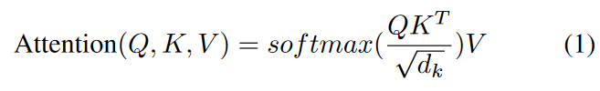
where Q is the query, K is the key, and V is the value. The scale factor √dk is intended to prevent the inner product from becoming too large, especially when the dimension is high. So, the attention function is achieved by computing the weights of the correlation, called the attention score, between the entire encoder sequence as key and value and a particular time step of the decoder as query. In particular, the self-attention module computes the attention score between different positions of the self sequence (i.e., Q=K=V) to compute the representation of the same sequence.
To allow the model to jointly note information from different representation subspaces at different locations, it further employs multi-head attention, defined as follows.
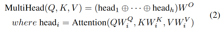
where W Q i ∈ Rdmodel×dq , W K i ∈ Rdmodel×dk , W V i ∈ Rdmodel×dv , W O ∈ Rhdv×dmodel is the learnable parameter matrix. The ⊕ denotes the concatenation operation. In our model, dmodel corresponds to the input dimension of the data, and we compute four parallel attention heads in the reduced dimension and concatenate them to the original dimension.
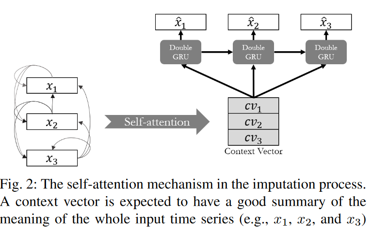
In this paper, the attention mechanism was employed to provide more targeted clues to the imputation problem for two reasons. First, it allows the model to pay attention not only to temporal sequences but also to time steps with relatively similar patterns. This is particularly appropriate for time series with periodicity. Many time series may have periodic properties in their sequences (e.g., weather forecasts, traffic predictions, etc.). Second, sufficient information can be obtained from the entire sequence, not just a few time steps back and forth. If the series has many missing values, the quality of the information provided by the entire line is better than from only a few time steps. This property is difficult to capture with conventional methods (RNN methods) that rely on a time sequence. Therefore, in our model, as shown in Fig. 2, we transform the input sequence into a context vector (i.e., Q and K are obtained from the same input sequence) using the self-observation module and consider the quantitative correlation of the entire series. We then design a temporal attention module that reflects the correlation between the hidden state of the GRU and the context vector (Q is the hidden state and K is the context vector).
The Temporal decay layer controls the effect of past observations at irregular time intervals in the GRUs. The decay rate must be learned from the data since it varies from variable to variable based on the underlying properties associated with the variables, as missing patterns are unknown and potentially complex. That is, the vector of attenuation rates γt at t is defined as follows
where Wγ and bγ are learnable parameters and an exponential negative rectifier is used to ensure that each decay rate is monotonically decreasing in the range 0 to 1. As long as these conditions are satisfied, the functions can be replaced by others. Intuitively, the effect is to attenuate features extracted from the hidden state rather than directly from the raw input variables. By learning how much previous information the hidden state has is attenuated and used, the attenuation rate adjusts the previous hidden state (ht-1) to h′t-1 by an element-by-element multiplication before entering the GRU-cell.
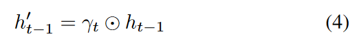
Here is the element-wise multiplication.
B. Identifier
Similar to the GAN framework, we introduce a discriminator (D) as an adversary to train G. D consists of a GRU module for time series processing, a fully connected layer for dimensionality reduction, and finally a sigmoid activation that produces the probability of each element as an output. Since D has been experimentally found to converge relatively easily, we use a simpler structure than G for stable adversarial learning. The loss function for learning D is also relatively simple: for the same reasons as for G, we could not apply the traditional Wasserstein GAN loss as is: the input to D is the matrix ˆ X imputed by G, which is a combination of values imputed as elements and observed values. That is, each corresponds to a false value or a real value. This means that the loss function must simultaneously consider both types of inputs in the matrix. For this reason, we define the loss function (LD) of D as

The first term shows the loss when D takes a false value as input and the second term shows the loss when D takes a real value as input. Since forward G and backward G each produce a matrix as an output, D also has two losses corresponding to both. However, we show only one for convenience.
C. Finding the optimal noise
Much of the work with GANs aims to generate realistic multiple samples by varying a random vector z, called "noise". However, this approach may not apply to the Imitation problem. That is, it needs to successfully perform the two tasks of not only filling in the missing values but also matching the observations exactly. Due to this specificity, z-search plays an important role. Specifically, the random noise vector z is randomly sampled from a latent space such as a Gaussian distribution. This means that as the input random noise z changes, the generated sample G(z) changes significantly. Even if the generated sample follows the true distribution of the original data, the similarity between x and G(z) may not be sufficiently large. That is, although their distributions are similar in a broad sense, individual samples may differ significantly in a particular view. To address this issue and further improve the similarity, finding the best matching optimal noise z′ is introduced. Since we already know some of the conditions (observed values in the samples), we can use them to iteratively find a more appropriate z. This method has been widely applied in the field of image data texture transformation, inpainting, and tabular data imputation.
Inspired by these studies, our model searches for the optimal noise z′ by learning at the inference stage, which generates more suitable missing values for samples on the distribution of the original data. Learning in the inference stage does not learn the parameters of the model, but backpropagates over the input zt that is updated at each iteration. zt learning uses the same loss as the learning G (LG) in (9). That is, we iteratively update the gradient - ∂LG/∂zt and search for a more suitable one. After searching for the best noise z′t as one of the inputs, we generate two imputed matrices by forward and backward G, respectively. Finally, the average of the two matrices is used to determine the final imputed result.
experiment
In this section, experiments are conducted to prove the validity of the proposed STING model by answering the following research questions
- RQ1 Is STING superior to other state-of-the-art imputation methods?
- RQ2 How does STING act on downstream tasks as a post-imputation?
- RQ3 Which modules have the greatest impact on STING's performance improvement?
In the following, we first describe the dataset and baseline methods used in our experiments. Next, we compare the proposed STING with other comparative methods and provide a detailed analysis of STING under two different experimental settings. Finally, a truncation study is conducted to analyze the impact of the main modules of STING.
For all datasets, min-max normalization was applied during the experiment for the details of the basic experimental setup. All experiments were repeated 10 times and the average accuracy was reported, taking into account any kind of randomness during the experiment. The generators were pre-trained for 10 epochs with LR and LC in (6) and (7). We found experimentally that pre-training the generators a little bit in advance allows them to converge faster and perform better. We then alternated updating the generator and discriminator one by one at each iteration. The models were trained using the Adam optimizer. The learning rates of the generator and discriminator were 0.001 and 0.0001, respectively. The ratio of hints given to the discriminator was fixed at 0.1. The batch size was set to 128. We set λr and λc to 10 and 1, respectively, as hyperparameters for the loss in (9). The model was implemented in PyTorch and all training was done on a single 2080Ti GPU with 11GB RAM.
A. Datasets
PhysioNet Challenge 2012 Dataset (PhysioNet) - Derived from PhysioNet Challenge 20121, this dataset aims to develop patient-specific prediction methods for in-hospital mortality. It consists of 12,000 multivariate clinical time series records from intensive care unit (ICU) stays. We use training set A (4,000 ICU stays) of the entire dataset. The experimental preprocessed dataset has a total of 192,000 samples. Each sample contains 37 variables such as DiasABP, HR, Na, and Lactate over 48 hours. There are 554 patients (13.85%) with positive death labels. This dataset has a high missing rate (80.53%) and is very sparse, making it difficult to perform downstream tasks such as mortality prediction simply. Therefore, many previous studies have experimented with this dataset to evaluate the performance of imputation and post-imputation tasks.
KDD CUP Challenge 2018 Dataset (Air Quality) - Accessible from the UCI Machine Learning Repository, the KDD CUP Challenge 2018 Dataset (Air Quality) is a public air quality dataset, used in the KDD CUP Challenge 2018 to accurately predict the Air Quality Index (AQI) for future 48 hours. The records have a total of 12 variables, including PM2.5, PM10, and SO2 from 12 monitoring stations in Beijing. The period was from March 1, 2013, to February 28, 2017, and variables were measured hourly. The total sample size is 420,768 with some missing values (1.43%).
Gas Sensor Array Temperature Modulation Dataset (Gas Sensor) - Accessed from the UCI Machine Learning Repository. the dynamic mixture of carbon monoxide (CO) and moist synthetic air in a gas chamber for 3 weeks. Includes 14 temperature-modulated metal oxide (MOX) gas sensors exposed to a dynamic mixture of carbon monoxide (CO) and moist synthetic air in a gas chamber for three weeks. One day of the total data set is used for the experiment. The number of samples is 295,704. Each sample consists of 20 variables, including the CO concentration in the gas chamber. Unlike other data sets, all samples are fully observed.
B. Baselines
To evaluate the performance of our model, we compare it to the following representative baselines. Statistics-based (Stats-based), Machine Learning-based (ML-based), and Neural Network-based (NN-based). The ML-based model was implemented based on the python packages sklearn and f ancyimpute. The NN-based model hyperparameters and other experimental settings were set up according to the corresponding papers, respectively.
- Mean simply fills the missing value with the global mean of the corresponding variable.
- Prev Fill (Prev) fills the missing values with the previously observed values. This method is a very simple and computationally efficient imputation due to its time series nature.
- KNN [35] uses K-Nearest Neighbors to find 10 similar samples and fills the missing values with the average of these samples.
- Matrix Factorization (MF) [36] is a method that directly factors an incomplete matrix into two low-rank matrices solved by gradient descent and imputes missing values by matrix completion.
- Multiple Imputation by Chained Equations (MICE) [10], [37] iteratively models each feature with missing values as a function of other features and imputes using their estimates.
- Generative Adversarial Imputation Nets (GAIN) [18] impute missing values conditional on what is observed using GANs.
- Gated Recurrent Unit with Decay (GRU-D) [2] is based on GRU and imputes missing values using a decay mechanism at irregular time intervals.
- E2GAN (End-to-End Generative Adversarial Network) [16] is based on GAN and is characterized by the fact that the generator has an autoencoder structure. That is, it can optimize low-dimensional vectors while learning the distribution of the original time series.
- Bidirectional Recurrent Imputation for Time Series (BRITS) [15] adapts a bidirectional RNN to embed missing values without any specific assumptions on the dataset.
C. Direct Evaluation of Imputation Performance (RQ1)
The purpose of this experiment is to directly evaluate the imputation performance between the baseline and the STING. In this experiment, a certain percentage of observations were randomly eliminated and used as ground truth. The remaining observations were then used as training data for the imputation models. Once the replacement training for each model was completed, we replaced the missing values via each model and inferred the complete data. We then compared the inferred values to the ground truth and measured the performance of each model using RMSE (Root Mean Squared Error), with smaller values indicating better performance. In the first experiment, we set the ratio to the truth value to 20% and compared the performance of all models on the three datasets; in the second experiment, we varied the truth ratio from 10% to 90% and evaluated the best-performing baseline performance.
Table I summarizes the results of the first experiment, where we see that STING achieves the best performance on all datasets. Compared to the best performing baseline (i.e. BRITS), the error improvement of the results is 4.0%, 21.0%, and 59.1%, respectively. One statistical method, Prev, performs quite well. This indicates that simply substituting in past values may perform better than other models that are time-consuming and complex. This is reasonable due to the nature of time series data collection and its heavy reliance on past samples. In particular, for data sets with little temporal variation, filling in with past values can yield significant benefits at little cost. Prev also shows similar performance trends to GRU-D. This makes a lot of sense because GRU-D learns the ratio of mean to historical values and fills in the missing values. Among the ML-based models, KNN shows the best performance similar to BRITS on the gas sensor dataset, but its performance is not stable on other datasets. On the other hand, MICE shows relatively good and stable performance on all datasets, while GAIN based on GAN does not show good performance on the time series dataset due to the lack of a suitable learning strategy for time series.
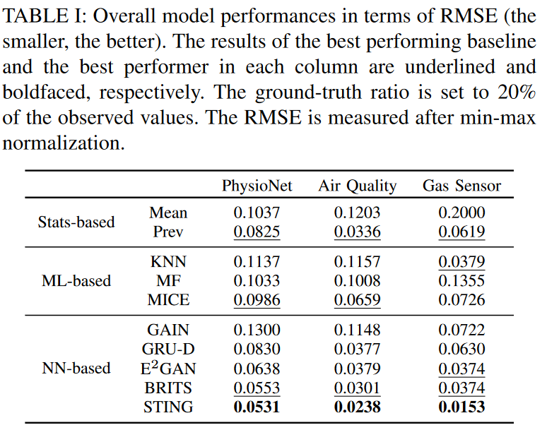
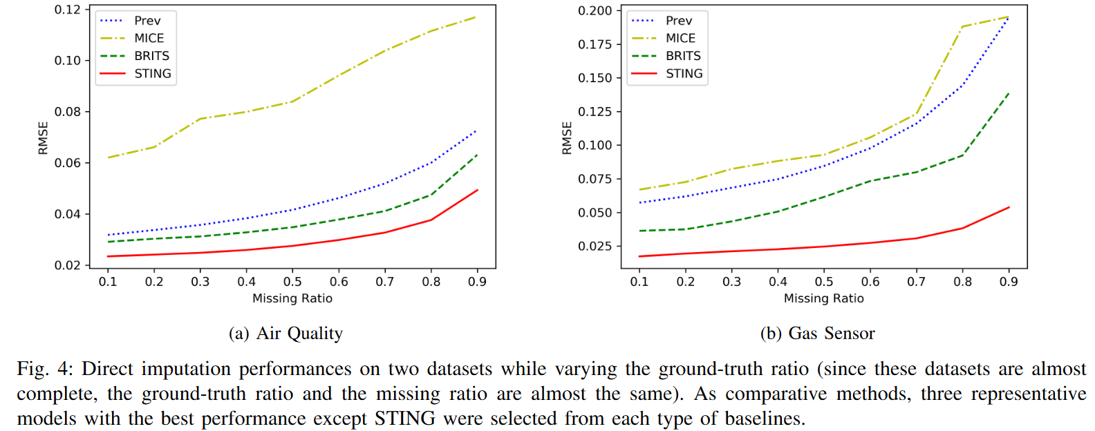
Fig. 4 shows the performance results of the second experiment for varying the missing fraction of the two datasets. Note that PhysioNet is excluded from this experiment because it has a very high missing fraction (80.53%). A high missing rate, on the contrary, reduces the training data used for imputation training and thus reduces the performance of all models. Nevertheless, we can see that STING achieves the best performance in all conditions, with gradual performance degradation. In other words, the more the dataset contains missing values, the less sensitive STING is to the imputation of missing values compared to others. This result confirms that STING exploits the attention mechanism since relatively more information is available by referring to the whole sequence.
D. Indirect Evaluation of Imputation Performance (RQ2)
The purpose of this experiment is to evaluate the performance of imputation indirectly by the solution results of the downstream task. If the distributions of the original data and the imputation data are similar, the results of the downstream task should also be similar. Therefore, we can indirectly see how much imperfect data was imputed through the prediction results. For stable training of the prediction model, we only use the gas sensor dataset, which is originally complete data. This data also allows us to assume an ideal replacement model where all missing values are replaced by ground truth, thus obtaining an upper-bound prediction performance. In this experiment, this ideal replacement model is also included as a baseline. Note that we do not train the imputation and prediction tasks at the same time in this experiment, since our goal is to measure the imputation performance, not to improve the prediction performance. After imputing the non-label test data, they are inferred by the prediction model learned on the full training data, which has already been trained. This is intended to provide a fair comparison of models in a typical setup where labels are not clear or missing.
The procedure of this experiment is as follows. To set up the imputation and regression models independently, we first divide the dataset into 80% training data and 20% test data. Using this complete training data, we first train a regression model to predict the target CO concentration. For the regression model, we built a simple GRU with two layers and a dropout of 0.3, and finally a fully connected layer. Then, the training data was made to have completely random missing values in a certain ratio. After training our method and baseline on the training data, the missing values other than the target of the test data can be imputed by the obtained model to obtain different imputed test data sets corresponding to each model. Then, based on the imputed test data, the target is predicted using regression models. Finally, the RMSE results between the predicted and actual target values are measured. This evaluation method allows us to determine whether the imputed data follows the distribution of the original data under the assumption that similar distributions yield similar performance. In other words, by comparing how close the original test data is to the regression results (as imputed by the ideal model), we can determine which imputed data is closer to the true distribution. It is important to note that we do not aim to achieve state-of-the-art predictive performance.
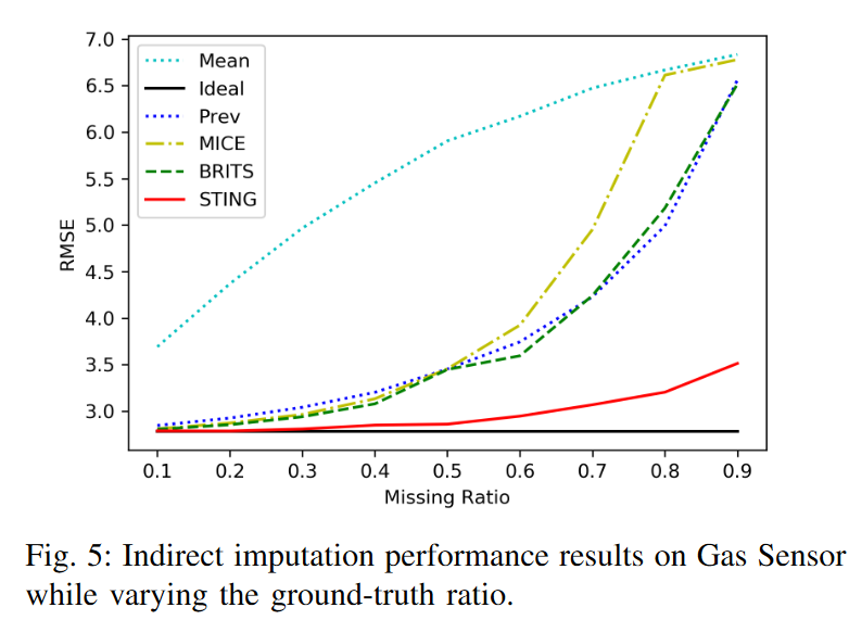
Fig. 5 shows the RMSE results of the regression model for each imputed data while varying the ground truth ratio. We can see that the ideal model has the lowest and constant RMSE because it can impute the original test data at any missing ratio. Among the imputation models compared, STING achieves the best performance at any ratio. Mean, on the other hand, performs the worst, showing how inefficient it is to impute time series with mean values. Interestingly, there is a clear difference between missing ratios of about 0.5. Previously, most models maintained similarly good performance below 3.5, but then the RMSE increases dramatically. For a grand truth of 0.9, STING shows a relatively small increase in error despite the poor conditions; there appears to be an advantage to using GANs to generate new time series and using information from the entire sequence through the mechanism of attention.
E. Ablation Study (RQ3)
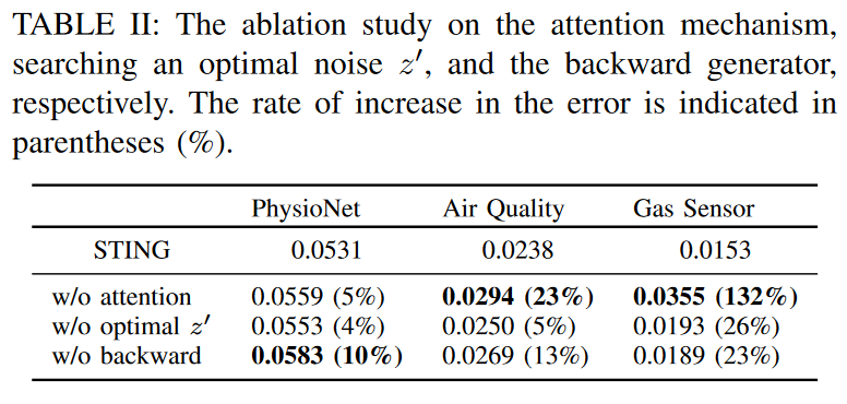
Potential sources of STING's effectiveness are the two attention modules, the optimal noise z′ search method, and the backward generator, respectively. To understand how each key feature affects the performance improvement of STING, we performed ablation experiments and compared the performance of the resulting architecture with the overall STING architecture. To this end, we experimented with three models in three datasets, each excluding only one feature from STING. We measured the RMSE at the imputed values by setting the ratio of ground truth to 20% of the observed values.
Table II shows the ablation results, with an increase in RMSE in all cases. The results with the backward generator removed to show the highest increase in error rate for PhysioNet. On the other hand, the results with the attention module were removed to show the highest increase in error rate for Gas Sensors and Air Quality. This suggests that the proposed attention module plays a relatively important function in STING. Namely, in the process of learning the correlation across sequences, it generates significantly important information for imputation on any dataset. On the other hand, the module that searches for the optimal noise z′ has a relatively small effect. This shows that even if z is randomly generated, it is still possible to produce samples that match well with the actual distribution of the original data since the observed values of X are conditioned on G in STING. In other words, even with suboptimal noise STING may be able to efficiently learn the distribution of the original time series, and this process plays a complementary role.
The above comparison experiments with other models have demonstrated the effectiveness of the STING. Two main factors contributed to the remarkable performance even under poor conditions. First, we confirmed that the GAN mechanism works well and produces samples that follow the true distribution of the original time series; we illustrated how STING, when set up, converges to the desired distribution. In particular, we explained that the discriminator problem is set more delicately at the Wasserstein distance to maximize the adversarial learning effect, comparing it with previous work using GANs. As a second key factor, we found that the proposed attention mechanism was effective in the imputation task: STING was able to acquire more information by focusing on certain periodic patterns or certain time steps. This effect became more pronounced as the missing rate increased, clearly demonstrating the advantage of retaining a large amount of information during imputation.
summary
In this paper, we propose STING, a novel imputation method for multivariate time series data based on generative adversarial networks and two-way recurrent neural networks to learn latent representations of time series. We also propose novel self- and time-imputation mechanisms to capture weighted correlations across time series and prevent potential biases from irrelevant time steps. Various experiments on real-world datasets show that STING outperforms previous state-of-the-art methods in both imputation accuracy and downstream performance with imputed values. In the future, they plan to investigate imputation on more general data, including categorical types; for GANs, generating categorical data is a particularly challenging problem, and testing the potential of GANs to generate and impute categorical data is a topic for future research.


Categories related to this article


