
New Trends In Time Series Analysis : Robust Time Series "Chain" Extraction By Incremental Nearest Neighbor Method TSC22
3 main points
✔️ A relatively new method of finding characteristic "chains" in time series data has been powerfully updated
✔️ The algorithm accurately finds "chains" as the data changes and is robust against noise
✔️ Qualitative evaluation on real-world data and quantitative evaluation on synthetic data have Excellent performance has been confirmed
Robust Time Series Chain Discovery with Incremental Nearest Neighbors
written by Li Zhang, Yan Zhu, Yifeng Gao, Jessica Lin
(Submitted on 3 Nov 2022)
Comments: ICDM 2022
Subjects: Machine Learning (cs.LG); Artificial Intelligence (cs.AI); Information Retrieval (cs.IR)
code:

The images used in this article are from the paper, the introductory slides, or were created based on them.
summary
There are many approaches to analyzing and modeling time series data, and the "Time Series Chain (TSC)" introduced here is a relatively new method among them.
The discovery of time series motifs has been a fundamental challenge for the identification of meaningful repeating patterns in time series data. Recently, time series chains were introduced as an extension of time series motifs to identify continuously evolving patterns in time series data. Informally, a time series chain (TSC) is a temporally ordered set of time series sub-sentences, where every sub-sentence is similar to the one before it, but the last and the first can be arbitrarily dissimilar.TSCs can reveal potential continuous evolving trends in time series and identify anomalous phenomena in complex systems They can identify precursors of anomalous phenomena in complex systems. Unfortunately, however, existing definitions of TSC do not accurately cover the evolving portions of a time series. The discovered chains are easily broken by noise and may contain non-evolving patterns, making them impractical for real-world applications. Inspired by recent work tracking how recent neighborhoods of time series subsequences change over time, we introduce a new definition of TSC that is more robust to noise in the data in the sense that it can better find evolving patterns while excluding non-evolving patterns. In addition, we propose two new quality metrics to rank the discovered chains. Through extensive empirical evaluation, we demonstrate that the proposed definition of TSC is more robust to noise than previous techniques and that the top discovered chains can reveal meaningful regularities in a variety of real-world data sets.
Introduction.
Over the past two decades, the task of finding repeating patterns in time series data, known as motif discovery, has received much attention in the research community due to its wide range of applications across many different domains. Recently, a new tool for capturing evolving patterns in time series data has been introduced, a primitive called time series chain (TSC). A time series chain is an ordered set of sub-sentences extracted from a time series such that adjacent sub-sentences in the chain are similar but the first and last are arbitrarily dissimilar. Unlike other time series data mining techniques such as motif discovery, discordance discovery, and time series clustering, time series chains can capture the latent drift that accumulates over time and is widespread in many complex systems, natural phenomena, and social changes.
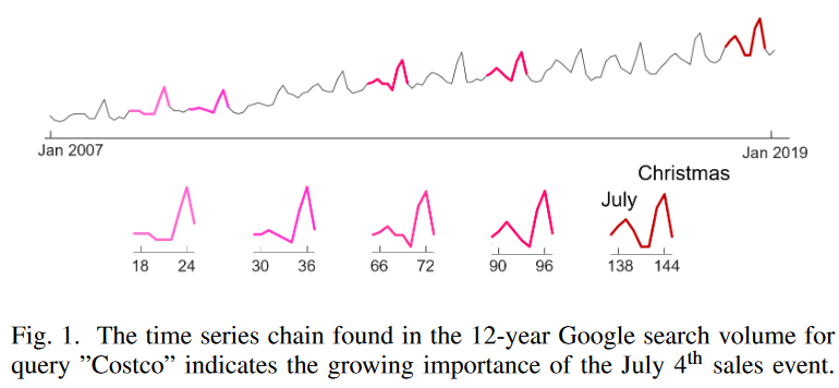
To better understand the function of time-series chains, consider the Google Trend data in Fig. 1 corresponding to 12 years of search terms for the American retail chain Costco. In the figure, the time-series chain found is highlighted. The first pattern in this chain shows a sharp peak around Christmas. This is a normal pattern, as online shopping needs increase around the holiday season. Then, as that peak smoothes out over the years, a small bump appears around July, a pattern that gradually grows to become another major peak. This shifting pattern in the chain demonstrates people's growing interest in Costco's July 4th (Independence Day) online sales event and provides useful marketing insights.
Another typical application of time series chaining is prognostication. As noted in prior research, "most equipment failures are preceded by specific signs, conditions, or indications that such failures are likely to occur." Time series chains can identify not only a single antecedent, but also a series of patterns that reveal continuous and progressive changes in the system, helping the analyst find the cause early and prevent catastrophic failures. There are currently two methods for discovering time series chains. The concept of a chain was first introduced based on a bidirectional definition, and then a geometric definition was proposed to increase robustness. We will refer to the original time series chain definition as TSC17 and the later geometric chain definition as TSC20.
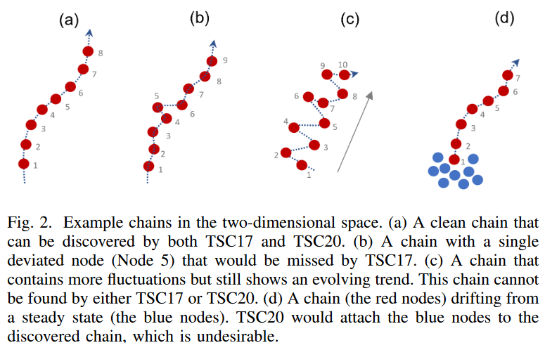
Despite the excellent interpretability of time series chains, unfortunately, it has been observed that existing chain discovery methods work well only in relatively ideal situations where the data are clean and the patterns unfold in small quasi-linear steps (as shown in Fig. 2.a). In practice, the continuous data collection process is often subject to environmental changes, human error, and interruptions in sensor signals. As a result, the data may contain noise, some patterns may deviate from the general trend (e.g. node 5 in Fig. 2.b), continuous patterns may be inverted, or the chain may develop a zigzag due to data fluctuations (Fig. 2.c). It may also remain relatively stable before the pattern begins to drift (as shown in Fig. 2.d, which is typical in prognostication). Existing chain discovery methods are not robust enough to handle such scenarios in real-world data.
Specifically, we found the following limitations in the existing definition of a time series chain
- The constraints introduced in TSC17 are too strict, and a small fluctuation can easily "break" the chain; Fig. 2.b shows an example that does not satisfy the constraints.
- The threshold for directional angle introduced in TSC20 is very sensitive to noise. If the data contain fluctuations, even a threshold of 50 degrees (the recommended threshold is 40 degrees) can miss apparent chains (e.g., Fig. 2.c). However, if the threshold is further increased, the discovered chains will contain many noisy patterns that have nothing to do with the evolving trend.
- Even when the directional angle is very small, the chains found by TSC20 may contain patterns that are unrelated to the evolving trend. For example, if data that was initially stable (very similar patterns) begins to drift (e.g. Fig. 2.d), TSC20 will add the stable (blue) pattern to the evolving chain. As a result, it is impossible to tell when the data started to drift.
To address these limitations, we propose a new time series chain definition, TSC22, that uses the idea of tracking how pattern nearest neighbors change over time to improve the robustness of chain discovery. like TSC17, TSC22 is a two-way definition, but the constraints are considerably relaxed and do not rely on angular constraints like TSC20. Furthermore, we propose a new quality metric to rank the chains discovered by this method. Empirical evaluations demonstrate that the proposed method is more robust to noise than previous methods and that the top chains discovered can reveal meaningful regularities in a variety of real-world data sets.
Related Research
Time series chaining is a relatively new topic. The most closely related work is by Zhu et al. and Imamura et al. Zhu et al. first introduced the concept of time series chains. In this study, all pairs of adjacent subsequences in a chain are forced to be the nearest neighbors on either side of each other, and the longest chain is reported as the top chain in the time series. While this concept is simple and intuitive, many real-world applications have shown that the requirement of bidirectional nearest neighbors is too stringent, as chains are easily broken by data fluctuations and noise. Imamura et al. relax the bidirectional condition by enforcing only a unidirectional left nearest neighbor condition and adding a predefined angle constraint to guarantee the directionality of the discovered chain. While this concept was shown to be more robust under some conditions, a new angle parameter was introduced and it was observed that in some real-world scenarios, no meaningful chains could be found no matter how this parameter was set.
Other studies on time series chains set the problem differently: Wang et al. explore ways to speed up chain discovery in streaming data using existing time series chain definitions; Zhang et al. propose a method to detect joint time series chains spanning two-time series Zhang et al.
The focus here is on improving the chain definition in a single time series.
Definition.
We first review the necessary time series notation and then discuss the formal definition of a time series chain.
A. Time series notation
This is a basic definition related to time series.
Definition 1. time series
T = [t1, t2, ..., tn] is an ordered list of data points, ti is a finite real number, and n is the length of the time series T.
Definition 2. time series subsequence
ST i= [ti, ti+1, ..., ti+l-1] is a continuous set of points starting from position i in time series T with length l. Usually l ≫ n and 1 ≤ i ≤ n - l + 1. , ti+l-1] is a continuous set of points starting at position i in time series T, of length l. Usually l ≫ n, and 1 ≤ i ≤ n - l + 1.
Subsequences can be extracted from a time series T by sliding a window of fixed length l between time series. Given a subsequence of the query, the distance to all subsequences of the time series T can be computed. This is called the distance profile.
Definition 3. distance profile
DQ,T is a vector containing the distances between the query subsequence Q and a subsequence of the same length in the time series T. Formally, DQ,T = [d(Q, S1), d(Q, S2), . , d(Q, Sn-l+1)], where d(. , .) denotes the distance function; in the special case where Q is a subsequence of the time series T starting from position i, we denote the distance profile by Di.
Following the original work of Matrix Profile, here we use z-normalized Euclidean distance instead of Euclidean distance to achieve scale and offset invariance.
In addition, the distance profile can be split into a left distance profile and a right distance profile.
Definition 4. left distance profile of a time series T
The DLi of a time series T is a vector containing the Euclidean distances between a given subsequence Si∈T and all subsequences to the left of Si. Formally, DLi = [d(Si, S1), d(Si, S2), . , d(Si, Si-l/2)].
Definition 5. right distance profile
DRi is the vector DRi = [d(Si, Si+l/2), . , d(Si, Sn-l+1)].
By examining the minimum values of the left and right distance profiles, respectively, one can easily find the left-side nearest neighbor (LNN) and right-side nearest neighbor (RNN) of a given subsequence. Two vectors, the left matrix profile, and the right matrix profile are used to store the distances between all subsequences and their corresponding left/right nearest neighbors, as well as the positions of their nearest neighbors.
Definition 6. left matrix profile
MPL is a 2-dimensional vector of size 2 × (n - l + 1), where MPL(1, i) = min(DLi) and MPL(2, i) = arg min(DLi).
where MPL(1, i) stores the distance between Si and the most similar subsequence before i (i.e., its LNN) and M PL(2, i) stores the position of the LN N
Definition 7. right matrix profile
MPR is a 2-dimensional vector of size 2 × (n - l + 1) where MPR(1, i) = min(DRi) and MPR(2, i) = arg min(DRi).
B. Definition of existing time series chain
All existing definitions of time series chains have been developed from backward time series chains and can be easily obtained given a left matrix profile.
Definition 8. backward chain of time series T
TSCBWD of a time series T is a finite ordered set of time series subsequences TSCBWD = [SC1, SC2, SC3, ..., SCm ], where C1 > C2 > ... C1 > C2 > ... > Cm is the index of the time series T such that LNN (SCi ) = SCi+1 for 1 ≤ i < m.
For the sake of clarity, we will refer to a part of the time series chain as a node. We will refer to the first node in the backward chain as the start node and the last node as the end node. Here, in TSCBWD, SC1 is the starting node and SCm is the ending node.
Similarly, a forward time series chain can be obtained from the right matrix profile.
Definition 9. forward chain
TSCFWD is a finite ordered set of subsequences of a time series T. TSCFWD = [SC1, SC2, SC3, ..., SCm ] where C1 < C2 < ... < Cm are indices of the time series T. For any 1 ≤ i < m, we do RN N (SCi ) = SCi+1.
Existing studies define chains by imposing different constraints on the backward chain; in TSC17, time series chains are defined based on the intersection of the backward and forward chains. This is called a bidirectional time series chain.
Definition 10. two-way time series chain
A two-way time series chain (TSC17) is a finite ordered set of subsequences of a time series T. TSC = [SC1, SC2, SC3, SCm ] where C1 > C2 > .... C1 > C2 > ... > Cm and for any 1 ≤ i < m we have LNN (SCi ) = SCi+1 and RN N (SCi+1 ) = SCi . where the size of the set m is denoted as the length of the chain.
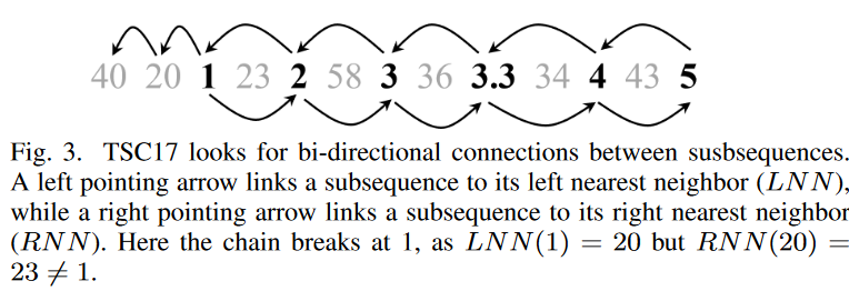
To understand how TSC17 works, consider the time series in Fig. 3.
40, 20, 1, 23, 2, 58, 3, 36, 3.3, 34, 4, 43, 5
The length of the subsequence is set to 1 and the distance is measured by the absolute value of the difference between the numbers. Follow the backward chain 5→4→3.3→2→1→20→40 to see if the LNN and RNN of each node can form a loop.
LNN (5) = 4 and RNN (4) = 5.
LNN (4) = 3.3 and RN N (3.3) = 4.
LNN (3.3) = 3 and RNN (3) = 3.3;
LNN (3) = 2 and RNN (2) = 3.
LNN (2)=1, RNN (1)=2.
LNN (1)=20 but RN N (20)=23 6=1, so the chain breaks at 1. As shown in Fig. 3, the extracted chain (retrograde) is
5 ↔ 4 ↔ 3.3 ↔ 3 ↔ 2 ↔ 1
A closer look at Fig. 3 reveals an excellent answer to this question. If one simply follows the chain 5→4→3.3→3→2→1→20→40 without any constraints, the chain loses its "directionality". The large noisy numbers (20, 40) simply do not fit the slowly decreasing trend; the bidirectional constraint in TSC17 removes these noisy signals from the chain.
In TSC20, time series chains are defined by applying angle constraints to the backward chain. This is called a geometric time series chain.
Definition 11. geometric time series chain of time series T
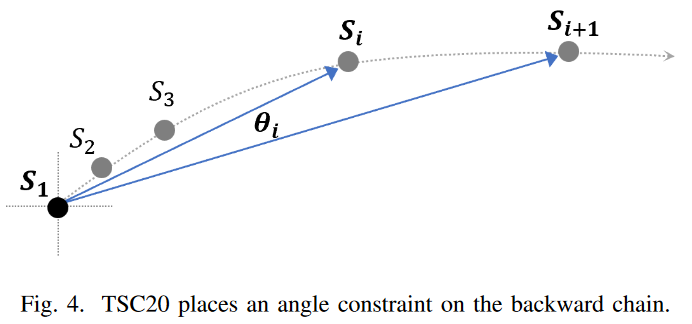
A geometric time series chain (TSC20) of a time series T is a finite ordered set of subsequences of a time series T. TSC = [SC1, SC2, SC3, ..., SCm ] (C1 > C2 > .... > Cm ) such that for any 1 ≤ i < m, we have LNN(SCi ) = SCi+1 and for any 2 ≤ i < m, we have i-th angle θi ≤ θ where.
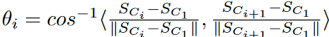
θ is a predefined threshold value.
Fig. 4 shows how the TSC20 definition works in 2-D space. The directional angle θi measures the change in direction from Si to Si+1 concerning anchor node S1. A small angle threshold between two consecutive subsequences of the chain ensures that the subsequences evolve in similar directions.
Limitations of TSC17 and TSC20
We find that both TSC17 and TSC20 are intuitive to use, but are susceptible to noise and fluctuations in the data.
A. Weaknesses of TSC17
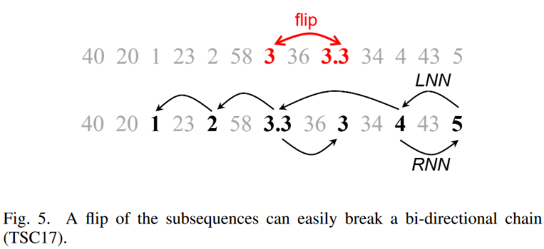
Let's look again at the example in Fig. 3, and Fig. 5. Suppose we invert the numbers 3 and 3.3, as shown above. Now the time series would look like this
40, 20, 1, 23, 2, 58, 3.3, 36, 3, 34, 4, 43, 5
Fig. 5. Consider extending the chain backward from node 5, as shown below: we see that LNN (5) = 4, LNN (4) = 5, so we can add 4 to the chain. Continuing, LNN (4) = 3.3, but RNN (3.3) = 3 6= 4, so we cannot add 3.3, and the chain breaks. However, from Fig. 5. below, we can see that we can create a reasonable chain that gradually decreases in the order 5 → 4 → 3.3 → 2 → 1, even when reversed. The two-way constraint is just too tight and the chain is not established.
B. Weaknesses of TSC20
The geometric chain definition used in TSC20 removes the bidirectional l constraint of TSC17 and uses only backward chains. While this results in longer chains, as shown in Fig. 3, irrelevant noise patterns can be included in the chains. To solve this, TSC20 adds an angle constraint on the backward chain. However, we found that this angle constraint created a new problem, as TSC20 missed obvious chains in some situations and added unwanted patterns to the found chains in others.
1) Overlooking an obvious chain of events
Fig. 6. Consider the two-dimensional example above. Assume that the subsequences appear in the following order in time
s9, s8, s7, s6, s5, s4, s3, s2, s1
The partial sequence is evolving in a zigzag fashion, but the tendency to move slowly from left to right is visible. However, TSC20 cannot detect this linkage.
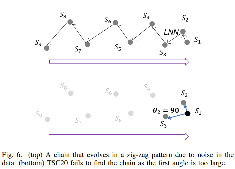
Following the TSC20 definition, in Fig. 6. top, we first find the backward chain starting from S1 (the arrows point all the subsequences to the LNN in 2D space), and then check the angles between successive subsequences based on the anchor subsequence S1. as shown in Fig. 6. bottom, the first angle θ1 = 90 degrees, and much larger than the threshold of 40 degrees proposed in TSC20, and the chain is immediately severed. We can check for all partial backward chains by reassigning the anchor to the next partial chain, but unfortunately, no partial chain satisfies the constraint.
Note that Fig. 6 only shows that fluctuations cause TSC20 to break down in two-dimensional space. In fact, in higher dimensional spaces, such evolving patterns are very common as noise and fluctuations cause the subsequences to drift in different directions.
2) Addition of undesirable patterns to the chain
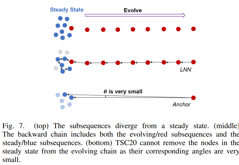
Another problem with TSC20 is that irrelevant patterns can be attached to the chain, degrading the quality of the chain; an example is shown in Fig. 7. above. Here, the subsequence is initially stationary (shown in blue) and then begins to drift to the right (shown in red). Ideally, the chain discovery algorithm would find all evolving (red) subsequences rather than the steady-state (blue) ones, so that the end node of the chain (the first red node on the left) would tell us exactly when the system begins to drift (i.e., the point of change). This temporal information is very important in prognostic applications because it helps identify the root cause of the drift. However, if we follow the backward chain shown in Fig. 7. we see that all successive nodes along this chain satisfy the angle constraint of TSC20. The red nodes are quasilinear and evolving, so their directional angles are close to zero. The angles corresponding to the successive blue nodes (Fig. 7. bottom) are also very small because these nodes are far from the anchor but very close to it. As a result, the TSC20 angle constraint cannot exclude the blue nodes from the chain and thus cannot detect the change point.
Proposed Method
To address the aforementioned limitations in the existing definition of time series chains, this paper proposes a new time series chain discovery method, named TSC22 As described in TSC20, a chain discovery method should consist of two parts. An algorithm to discover all chains in the data and a quality metric used to rank the discovered chains.
A. Incremental neighborhood
Our chain discovery method leverages the ideas of Y. Zhu et al. and tracks how the nearest neighbors of a time series subsequence change over time; Fig. 8 shows how this works, using the 1-dimensional running example from the previous section. Scanning from right to left to sub-array 2, the previous nearest neighbor sub-arrays (or incremental nearest neighbors) are stored based on the difference in their absolute values. We call the set {3, 4, 5} the incremental nearest neighbor set (IN N S) because it shows how the position of the nearest neighbor of the sub-array changes when traversed from the end of the time series.
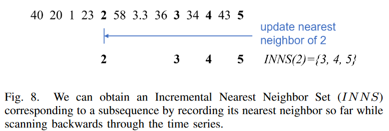
Definition 12 . the incremental neighborhood set (INNS) of a subsequence Si is the set of subsequences Sj (i<j≤n - l+1).
{Sj|d(Si, Sj) < d(Si, Sk) ∀k : j < k ≤ n - l + 1}
Note that the right neighbor of a subsequence is always included in the IN N S of the subsequence.
B. Find all chains in an incremental neighborhood
Based on incremental neighborhoods, we introduce a critical node, a key element in our definition of a chain.
Definition 13. A time series subsequence Si of a time series T is a critical node (CN) if Si ∈ IN N S(LNN (Si)).
Critical nodes can be based on more relaxed constraints than in Definition 10 (TSC17); since RNNs always belong to an incremental nearest neighbor set, nodes in the TSC17 chain are also critical nodes in this definition. We can find all critical nodes of a time series T . We call this the critical node set and denote it by CN T . This allows us to formally define TSC22 (relaxed-bi-directional time series chain).
Definition 14. a relaxed two-way time series chain (TSC22) of a time series T is a finite ordered set of time series subsequences.
T SC = [SC1 , SC2 , SC3 , ... , SCm ] , SCm ] (C1 > C2 > ... > Cm), such that: ... > Cm), such that:
1) For any 1 6 i < m, LN N (SCi ) = SCi+1, where
2) SC1 ∈ CN T,.
3) For any 1 < i 6 m, we have SCj ∈ IN N S(i), j = arg min i<j≤m SCj ∈ CN T
From condition (1), we see that our new chain definition TSC22, as well as TSC17 and TSC20, is built on top of the backward chain; we call it a "relaxed" bi-directional chain because the constraints on the forward chain are not as stringent as for TSC17.
Fig. 9 shows a one-dimensional time series as an example.
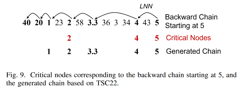
From (1) and (2), we see that TSC22 is a backward chain starting from a critical node. Now, let us expand the chain from node "5": as shown in Fig. 9, we find that LNN (5) = 4 and 5 ∈ IN N S (4) = {5}. This means that 5 is a critical node and a valid starting node for TSC22. Next, we move on to check the next node in the backward chain: 4 is a critical node since LN N (4) = 3.3 and 4 ∈ IN N S(3.3) = {3, 4, 5}; LN N (3.3) = 2, but 3.3 6∈ IN N S(2) = {3, 4, 5} so 3.3 is not a critical node, etc. Continuing the process, we see that the critical nodes on this backward chain are 5, 4, and 2. Condition (3) requires that for each node SCi in the chain (except the start node), the closest critical node in the chain that appears after SCi must be an element of IN N S(SCi ). Checking for each node in the backward chain 5→4→3.3→2→1→20→40, we see that partial chains 5, 4, 3.3, 2, 1 satisfy this condition, but partial chain 20 has 1 6∈IN N C(20) = {23, 34, 5} and the chain cannot break at this position. Therefore, the generated chain is 5 → 4 → 3.3 → 2 → 1. Essentially, condition (3) guarantees the "directionality" of the generated chain: as shown in Fig. 9, in both the original time series and the generated chain, subsequence 2 is closer to subsequence 1 than all subsequences to the right of 2, and in both the original time series and the generated chain, subsequence 4 is closer to subsequence 1 than all subsequences to the right of 4. Compared to the subsequences to the right of 2, subsequence 4 is closer to subsequences 2 and 3.3.
Comparing Fig. 9 with Fig. 5, we can see that TSC22 can extract meaningful chains even if some of the chain patterns are inverted due to noise. We also see that the zigzag chain in Fig. 6 can also be found by our definition. This indicates that TSC22 is more robust to noise than TSC17 and TSC20.
C. Ranking
Now that we have all the chains discovered in TSC22, we need a mechanism to measure their quality and rank them effectively; TSC17 ranks discovered chains by their length, which is not always effective, especially when there is a large amount of noise in the time series. in TSC20 As noted, TSC17 may find long chains even in stationary data that do not show an evolutionary trend, and the length of the top chains alone cannot determine if there are meaningful chains in the data. Ideally, a quality chain should have the following properties.
- High Divergence The first and last nodes in the chain must be sufficiently dissimilar.
- Gradual Change Successive nodes in a chain are very similar to each other.
- The Purity chain must not contain unrelated patterns.
- Length Longer chains are better for adequate coverage of drifting patterns.
Note that these quality views do not necessarily coincide. One chain may evolve very quickly, exhibit high divergence but low gradualism, and be short in length. On the other hand, another long chain could consist of patterns that are almost identical to each other but show no tendency to evolve. To address this, we develop two quality measures that take into account all characteristics and design a two-stage ranking algorithm based on these quality measures to ensure that high-quality chains stand out.
Effective length
Inspired by TSC20, we compute the "effective length" metric Leff, which simultaneously measures divergence and gradualism.

where b.e represents rounding to the nearest integer. The numerator is the distance between the first and last node of the chain and the denominator is the maximum distance between all consecutive pairs of nodes in the chain. If the chain evolves in a linear trace at a uniform rate, one can imagine that Leff is the length of the chain. This measure essentially indicates the approximate number of steps required to reach the end node from the start node when moving in a linear trace, with the distance per step being equal to the maximum continuous distance between the nodes of the chain. A chain with high divergence and gradualism should have a high Leff, while a chain containing noise should have Leff ≈ 1. Since Leff is an integer, there are ties. First rank the chains by their Leff scores, then perform a fine ranking based on the sum of squares of the correlations for the chains with the highest Leff scores.
Correlation length
The metric in this paper is called correlation length and is calculated as follows
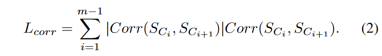
where Corr(.) is the Pearson correlation coefficient of the z-normalized subsequences, with values in the range [-1, 1]; if two subsequences are very similar, their Pearson correlation coefficient is close to 1; if they contain noise, it is usually smaller than 0.5. Here, the Pearson correlation coefficient is multiplied by its absolute value to magnify the difference between similar and dissimilar pairs. We call this measure correlation "length" because when successive nodes in a chain are very similar to each other, Lcorr is very close to the actual length of the chain. As a result, longer chains with highly similar subsequences will be prioritized in the fine-grain ranking phase. Compared to the TSC17 ranking method, which considers only chain length, and the TSC20 ranking method, which considers only divergence and gradualism, this ranking method has better coverage for all quality aspects of the chain. With the new ranking method and more robust chain definitions, TSC22 can effectively discover meaningful chains from various real-world and synthetic datasets, even in the presence of large amounts of noise in the data.
experimental evaluation
We demonstrate that the proposed method is more robust than the current state-of-the-art time series chain discovery methods, TSC17 (ICDM'17) and TSC20 (KDD'20), on both the real-world and synthetic data. To ensure a fair comparison, we use the original Matlab source code for both TSC17 and TSC20, and the default direction angles for TSC20.
We first analyze the performance of the three chain discovery methods qualitatively through several case studies on real-world data, and then make quantitative comparisons on a large synthetic dataset for which we can compute performance measures based on absolute ground truth.
A. Case Study: Robust Analysis of Penguin Activity Data
1) Clean data
Here we use the penguin activity time series from Y. Zhu et al. This shows the x-axis acceleration of the bird as it moves. The length of the sub-sequence is 25; Fig. 10 shows 22.5 s of data (recorded at 40 Hz) as the penguin dives into the water. The bird reaches the surface of the water about 2 seconds later (80th data point), after which the depth values begin to increase; as shown in Fig. 10, TSC22 is a high-quality chain with the first peak slightly lower than the second peak, the first peak getting higher with time, and the second peak getting weaker We found a high-quality chain that shows an evolving trend. This chain shows how the penguins adjust their flapping to balance the increase in buoyancy and water pressure; the chain obtained with TSC22 covers the entire diving range, while the chain obtained with TSC20 is missing a few nodes at the end and the chain obtained with TSC17 a few nodes on both sides. 20 and TSC17 chains can show the evolutionary trend of the pattern but are not able to show the start/end time of the evolutionary procedure.
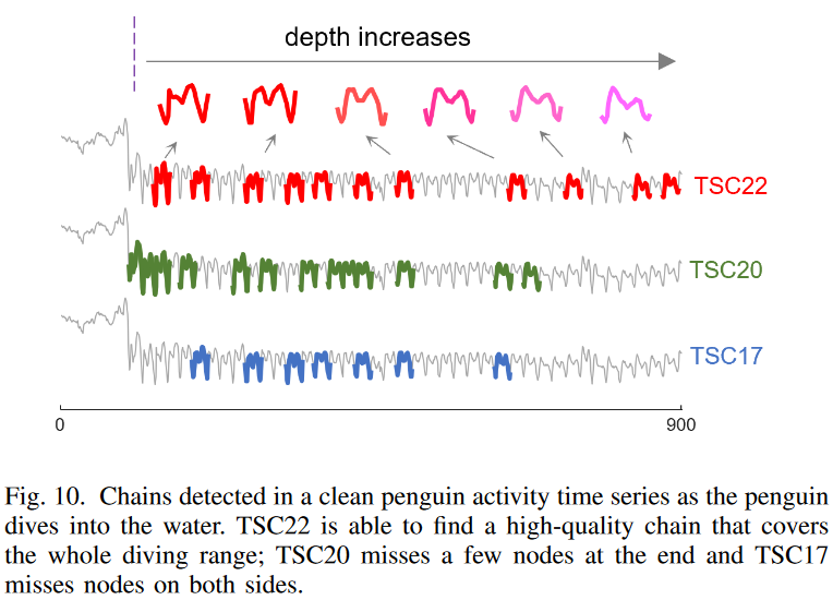
One might wonder if the inability of TSC17 and TSC20 to find the TSC22 chain in Fig. 10 is due to the constraints of TSC17 and TSC20, or to a ranking mechanism that favors other chains over the TSC22 chain. A closer inspection reveals that the TSC22 chain does not satisfy either the TSC17 or TSC20 definitions; as in Fig. 5, due to natural fluctuations in the data (e.g., the possibility that the penguins changed their direction of movement to avoid other animals), most of the contiguous nodes on the chain are not found in the TSC 17 two-way nearest neighbor constraint is not satisfied. Then, following the TSC22 chain in reverse, we see that the directional angle formed by the first three nodes in this chain (see Fig. 6) is 114 degrees, well above the TSC20 angular threshold (40 degrees), so the chain is broken instantly. This example validates the weakness of TSC17 and TSC20 in high-dimensional real-world data with natural fluctuations and demonstrates the robustness of TSC22 in such data.
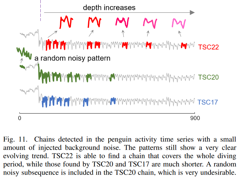
2) Data with Lydam background noise
In Fig. 11, to further test the robustness of the three methods, a small amount (±0.08 magnitude) of random noise is added to the penguin data to simulate additional background noise from the sensor. In this case, we see that TSC22 still finds high-quality chains across the entire diving procedure, and the patterns found show a very clear evolutionary trend even in the presence of additional noise. However, TSC20 and TSC17 failed to capture this chain, and their top chains now cover only half of the evolving range. Furthermore, TSC20 adds a random noise pattern to its top chain. This represents a weakening of the ability to filter out directional angle constraints as the backward chain gets longer.
B. Case Study: Detecting change points in scatter and table data
Here we compare how the three methods under consideration perform when the system transitions from a steady state to a drift state using the tilt table data of Y. Zhu et al. Fig. 12 shows the arterial blood pressure (ABP) signal of a patient lying on the tilt table. Here, the length of the partial array is set to 180, which roughly corresponds to a cardiac cycle. We find that such data are typical of many other areas, especially in prognostication, where the system initially operates in a stable state and then begins to deteriorate. It is therefore important to correctly identify the point of change (the beginning of the drift) so that the information can be used to determine the implicit mechanism that caused the drift and prevent system failure earlier.
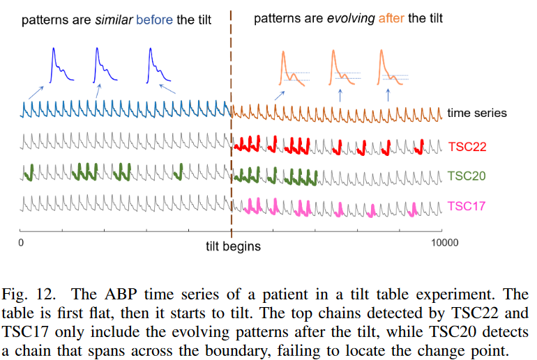
Looking at Fig. 12, we can see that TSC22 and TSC17 succeed in finding chains only for the right-hand portion of the post-tilt data, while TSC20 detects chains that span the tilt and stationary portions of the data. In this case, it is not hard to understand why TSC20 fails to produce pure chains (see Fig. 7). Since any pair of pre-tilted subsequences concerning the anchor point is nearly identical, the directional angle formed between them is close to zero; the unidirectional nature of TSC20 simply cannot stop backward chain growth when a stable interval of data is reached. On the other hand, the bidirectional restrictions in both TSC22 and TSC17 effectively stop those chains from growing into the stationary section. This example further illustrates the usefulness of TSC22: TSC22 can pinpoint exactly when the system begins to drift, making it easy for the analyst to find the implicit cause of the drift by examining events occurring before and after it.
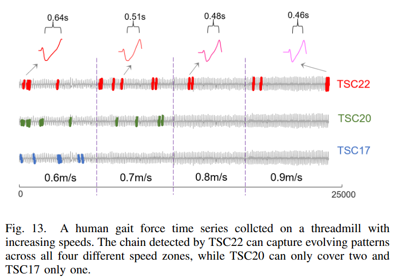
C. Case Study: Chain Discovery in Multiple Training Stages on Human Gait Force Data
The human walking force time series was used to evaluate the chain-finding method. As shown in Fig. 13, this time series represents the backward and forward forces detected by the sensors on a split-belt treadmill operating at four different running speeds. From Fig. 13, the chains detected on the TSC22 were all spanning different speed zones. The sharply indented pattern of the chains indicates that the force changes more rapidly as the speed increases and the subject's feet spend less time on the thread mill floor. The shorter dip-to-peak time also indicates a faster running speed. However, TSC20 and TSC17 can only detect chains in part of the data and cannot cover the full range, even though the pattern evolves over the entire time series.
In this case, why do TSC20 and TSC17 fail? Note that the patterns within the same speed zone are relatively similar to each other and evolve at a fairly small pace because the speeds are increasing piecemeal and constant. Since there are natural fluctuations in the participants' movements, many patterns within the same speed zone are reversed (see Fig. 5), and the overall evolution is closer to a zigzag chain like Fig. 2.c or Fig. 6, rather than the one in Fig. 2.a. As a soundness check, we can see that none of the nodes on the TSC22 chain in Fig. 13 satisfy the bidirectional nearest neighbor constraint of TSC20, and the directional angle formed by the last three nodes on the chain (i.e., the first three nodes of the backward chain) is 86 degrees, far exceeding the TSC20 angle limit of 40 degrees. This example further demonstrates the excellent robustness of TSC22 for real-world time series data, which naturally have many fluctuations and noise.
D. Quantitative Robustness Analysis
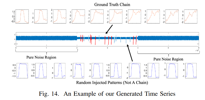
In the above evaluation, there are no absolute ground-truth labels (i.e., the exact location of each pattern in the chain in the time series), and the potential ambiguity of these labels make it difficult to perform a reasonable quantitative analysis based on real-world data. Therefore, to calculate quantitative performance measures such as accuracy and recall, we created a large synthetic dataset and manually embedded chain patterns into it to test whether the three methods in question could accurately locate these patterns.
Fig. 14 is an example of the time series created. Here, the first node of the ground-truth chain (Fig. 14. top) is randomly sampled from a dataset in the UCR Time Series Classification Archive1 and the last node is a random walk pattern. The chain consists of 10 nodes and evolves linearly from the first node to the last. The nodes of this chain are embedded in random positions while maintaining their order in the random noise time series. To increase the difficulty of the task, we added random noise on top of the data to distort the pattern and also embed 10 patterns (shown below in Fig. 14.) in the time series that are similar to the first node (sampled from the same data set) but unrelated to the evolving trend. Two random noise sections were added at the beginning and end of the generated time series to simulate a real-world scenario where the chain does not extend over the entire time series. To construct the synthetic time series, we used 17 datasets from the UCR time series archive, covering all sensor, ECG, and simulation shape data with instance lengths from 50 to 500, omitting datasets containing high-frequency patterns that would make a visual interpretation of the generated chains difficult The data sets containing high-frequency patterns that would make a visual interpretation of the generated chains difficult were omitted. For each dataset, we generated five different time series and measured the average performance of each chain discovery method on these time series.
A hit is defined as a hit if the nodes (i.e., subsequences) of the detected chain overlap the ground truth by 50% or more.
Since all TSC methods consist of two steps, chain detection, and ranking, experiments were conducted to compare performance with and without the ranking step.
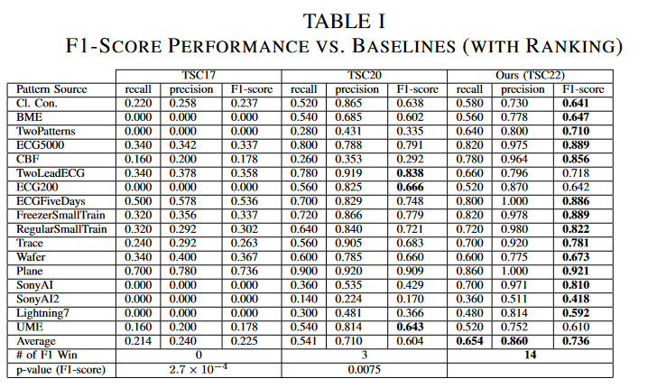
1) Overall performance when using rankings
Table I shows the performance of the top 1 chains detected by the three methods; TSC22 has a higher F1 score than both baselines in 14 of the 17 data sets, with a mean value (0.736) much better than TSC17 (0.225) and TSC20 (0.604). The p-value of the Wilcoxon signed-rank test between TSC22 and TSC17 was 2.7 × 10⁻⁴ and between TSC22 and TSC20 was 0.0075. Both p-values are less than 0.05, indicating that TSC22 is statistically significantly better than the baseline.
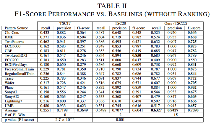
2) Performance without ranking
To fairly compare the three TSC methods using a definition that eliminates the influence of ranking, we fixed the starting node of the chain and evaluated the performance of the discovered chains. In each time series, we "grew" the chain independently from the last five nodes of the grand-truth chain and reported the largest F1 score obtained among these five different chains. From Table II, we see that TSC22 outperforms both baselines in F1 scores in 15 of the 17 datasets The Wilcoxon test p Also since the p-value of the Wilcoxon test is less than 0.05, we can conclude that the definition of TSC22 is significantly better than the existing definition of TSC.
summary
We propose a new time series chain definition, TSC22, that improves the robustness of the chains against noise by using the idea of tracking how the nearest neighbors of a pattern change over time. In addition, two new quality metrics were proposed to effectively rank the detected chains. Extensive experiments on both real-world and synthetic data show that this new definition is much more robust than the state-of-the-art TSC definition. Case studies performed on real-world time series also showed that the top-ranked chains found by this method can reveal meaningful regularities in a variety of applications under different noise conditions.
(A powerful new tool has been proposed for time series data analysis, which has a wide range of applications. Readers are invited to evaluate their data.


Categories related to this article


