
Time Series Classification Dynamic Sparse Network DNS That Learns Over A Wide Receptive Field Without Complex Tuning
3 main points
✔️ This is a NeurIPS 2022 accepted paper. We propose a dynamic sparse network (DSN) with sparse connections for time series classification that can learn to cover various receptive fields without cumbersome hyperparameter tuning.
✔️ The kernel of each sparse layer is sparse and dynamic sparse learning can explore under constrained regions, thus reducing resource cost.
✔️ It is shown to achieve state-of-the-art performance on univariate and multivariate TSC datasets at less than 50% of the computational cost compared to SOTA. Furthermore, the proposed DSN method can be easily combined with other DST methods, demonstrating its effectiveness. This suggests future integration with superior methods.
Dynamic Sparse Network for Time Series Classification: Learning What to "see''
written by Qiao Xiao, Boqian Wu, Yu Zhang, Shiwei Liu, Mykola Pechenizkiy, Elena Mocanu, Decebal Constantin Mocanu
(Submitted on 19 Dec 2022)
Comments: Accepted at Neural Information Processing Systems (NeurIPS 2022)
Subjects: Machine Learning (cs.LG); Artificial Intelligence (cs.AI)
code:

The images used in this article are from the paper, the introductory slides, or were created based on them.
summary
In this paper, we propose a dynamic sparse network (DSN) for time series classification (TSC) that can be trained over a range of receptive field (RF) sizes without the need for hyperparameter tuning. The DSN model can be used on both univariate and multivariate TSC data sets to achieve recent state-of-the-art performance at less computational cost than baseline methods.
Introduction.
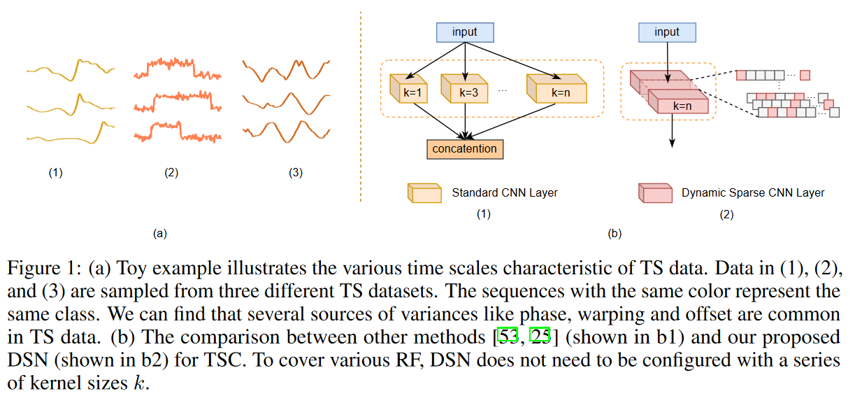
When collecting time series data, the challenge is to discover and take advantage of the various scaled signals hidden in the time series due to various variations in sampling rates, record lengths, and other factors. The main reason for this is due to several differences that naturally occur when collecting time series, such as sampling rate and record length. In addition, amplitude offsets, warps, and occlusions of data points are inevitable (see Fig. 1). Therefore, determining the optimal scale for feature extraction is difficult but important for the TSC task. One of the main solutions is to cover as many receptive field (RF) scales as possible so as not to ignore useful signals from the time series input.
Inspired by sparse neural network models that can perform as well as their dense counterparts with fewer connections, this paper proposes a sparse neural network model for the TSC task, consisting of a CNN layer with a large but dynamic sparse kernel that can automatically learn sparse connections in terms of covering various RF We propose a dynamic sparse network (DSN). The proposed DSN is trained by a dynamic sparse learning (DST) strategy, which also reduces the computational cost (e.g., floating point operations (FLOPs)) of learning and inference. While traditional dynamic sparse training methods search for connections layer by layer and can hardly cover small RFs, here we propose a finer sparse training method for TSCs. Specifically, the CNN kernels in each layer are partitioned into several groups, each of which can be explored under a constraint region during sparse training.
The main contributions of this paper are the proposal of a dynamic sparse network (DSN) for time series classification (TSC) that can learn to cover various receptive field (RF) sizes without the need for hyperparameter adjustment, and the reduction of computational and memory costs by dynamic sparse training To natively introduce a new DSN model for TSC that can be trained. The proposed DSN model achieves state-of-the-art performance on both univariate and multivariate TSC data sets with less computational cost than recent baseline methods.
Related Research
time series classification
The success of deep learning over the past decade has encouraged researchers to explore and extend its application to TSC tasks. In univariate TSC, deep learning-based models attempt to directly transform raw time-series data into low-dimensional feature representations via convolutional or recurrent networks. In multivariate TSC, LSTMs or attention layers are often stacked with CNN layers to extract complementary features from time series data. In recent years, since time series data consist of signals of various scales, many studies have attempted to extract features in a more scalable way. One of the main solutions is to configure appropriate kernels of various sizes to increase the probability of capturing the appropriate scale. Rocket-based methods aim to use random kernels of several sizes and extension factors to cover a variety of RFs in the TSC. Unlike these studies, the dynamic sparse CNN layer proposed here can adaptively learn a variety of RFs using deformable extension coefficients and trade-off both computational complexity and performance without cumbersome hyperparameter tuning.
sparse training
Recently, the lottery hypothesis has shown that it is possible to train sparse subnetworks to match the performance of their dense counterparts at a smaller computational cost. Instead of iteratively pruning from the dense network, recent work tries to find an initial mask to prune in one shot based on gradient information during training. After pruning, the topology of the neural network would be fixed during training. However, this type of model rarely comes close to the accuracy achieved by its high-density counterpart.
Introduced as a new learning paradigm before the lottery hypothesis, DST allows starting from a sparse network and dynamically evolving sparse connectivity with a fixed number of parameters during learning. Currently, DST is attracting attention from other research fields such as reinforcement learning and continuous learning, and its potential is believed to surpass the learning of dense neural networks. Unlike conventional DST methods, the proposed DSN learns with a fine-grained sparse learning strategy instead of the conventional layer-wise method to capture more diverse RFs in the TSC.
adaptive receptive field
RF which can be adaptively varied during learning has proven to be effective in many domains. Adaptive RF can usually be captured by learning the optimal kernel size or kernel mask during learning. However, since neither the kernel nor the mask is sparse, this can be computationally intensive when larger RFs are needed. Unlike these methods, the dynamic sparse CNN layer of DSN can be trained with DST and can learn to capture variable RFs using deformable expansion coefficients. Furthermore, the kernel is always sparse during training and inference, thus reducing the computational costs.
Proposed Method
problem definition
Definition 1. (Time Series Classification (TSC))
Let TS instance X = {X1,. Xn} ∈Rn × m, where m is the number of variates and n is the number of time steps. tsc predicts the class label y ∈ {1, . . c} from c classes exactly; if m equals 1, TSC is univariate; otherwise, it is multivariate.
Definition 2. (Time Series (TS) Training Set)
Training set D = { (X (1 ), y (1) ), ...., (X (N ), y (N) )}, where X(i) ∈ Rn×m is the label y (i) ∈ {1, ...., c} corresponding to univariate or multivariate TS instances.
Note here that all instances have the same number of time steps in the TS dataset. Without loss of generality, given a training set, the goal is to train a CNN classifier with adaptive and varied RFs for the TSC task at a low resource cost (e.g., memory and computation).
Dynamic sparse CNN layer with adaptive receptive fields
A simple strategy to cover a variety of RFs is to apply a multi-sized kernel at each CNN layer, but this has several limitations. First, TS instances from different TS datasets will most likely not have the same length and cycles, making it difficult to set up a fixed kernel configuration for all datasets even with prior knowledge. Second, to obtain a large receptive field, it is generally necessary to stack larger kernels and more layers, which increases storage and computation costs because more parameters are introduced.
To address these challenges, the proposed dynamic sparse CNN layer has a large but sparse kernel that can be trained to acquire adaptive RF. Specifically, given the input feature map xl ∈Rcl-1×h×w ( where h is 1 at univariate TSC and cl-1 is the number of input channels) and the kernel weights Θl ∈Rcl-1×cl×1×k ( where k is the kernel size and cl is the number of output channels) for layer l, the proposed dynamic sparse CNN layer The convolution by stride 1 and padding is formulated by

where Oj∈Rh×w denotes the output feature representation in the j-th output channel, Z denotes the set of integers, Il (-).Rcl-1×cl×1×k → {0, 1}cl-1×cl×1×k is the indicator function, Il (Θl)i,j denotes the activation weight of 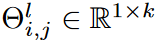 , the kernel of the (i, j)th channel,
  is element sum-product, and - denotes the convolution operator. The indicator function Il (-), which is learned when training the proposed DSN, satisfies
 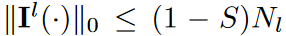 where 0≤S<1 is the sparse density ratio.
  denotes theL0 norm, Nl =cl-1×cl×1×k. When S > 0, the kernel is sparse, and using a large k in the dynamic sparse CNN layer yields a large RF with reduced computation.
Effective Neighbour Receptive Field size
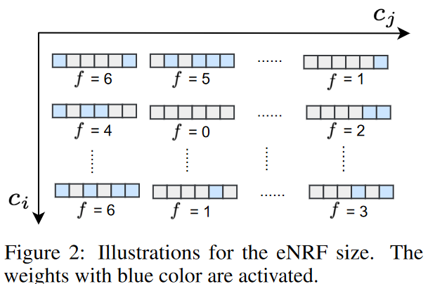
The receptive field is defined as the area in the input that is seen by the features in the CNN model. The region seen by each feature in each successive layer is defined as the Neighbour Receptive Field (NRF). Specifically, the size of the NRF corresponds to the kernel size of a standard CNN layer (considering the case where dilation is equal to 1). However, if the first or last weight in the kernel is not activated, the NRF size of the proposed dynamic sparse CNN layer will be smaller than the kernel size. For example, ∃i ∈ {1, .... cl-1}, j ∈ {1,. cl}, Il (Θl)i,j,1,1 = 0 or Il (Θl)i,j,1,k = 0. As shown in Fig. 2, eNRF size  of the kernel
  as the distance between the first and last activation weights in the l-th CNN layer,

Here  represents the set of indices corresponding to the nonzero weights of the kernel . This will be
 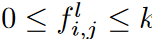 .
.
The eNRF size set for the lth dynamically sparse CNN layer is denoted F (l) and satisfies 0 ≤ min(F (l) ), max(F (l) ) ≤ k. Taking the case of the lth layer in Fig. 2 as a simple example, F (l) = {0, 1, 2, 3, 4, 5, 6}. Each dynamically perceiving CNN layer is considered to correspond to various eNRF sizes from 1 to k. If global information is expected, Il ( -) can be activated by distributing weights to obtain larger eNRFs and selectively use input features. On the other hand, when capturing local context, the weights to be activated tend to be concentrated because the eNRF is smaller; taking k = 5 as an example, Il (Θl)i,j could be [1, 0, 1, 0, 1] in the global context and [0, 0, 1, 1, 0] in the local context. Thus, the eNRF can be adaptively adjusted.
DSN Architecture
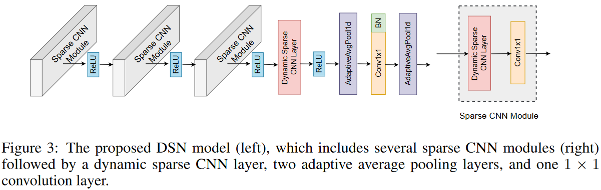
The proposed DSN model consists of three sparse CNN modules, each module consisting of a dynamic sparse CNN layer and a 1 × 1 CNN layer. Following the stacked sparse CNN modules are an additional dynamic sparse CNN layer, two adaptive mean pooling layers, and a 1 × 1 convolutional layer that serves as the classifier for the DSN model. The overall architecture is shown in Fig. 3.
Since the eNRF size of a 1 × 1 convolution is always equal to 1, the eNRF size set S(l) of the lth sparse CNN module is equal to that of the dynamic sparse CNN layer, and S (l) satisfies 0≤min(S (l)), max(S (l))≤k. Then, the eNRF size set of the three sparse CNN modules stacked consecutively can be described by RF as follows.

Equation (3) shows that the size of the RF can be increased linearly by stacking multiple sparse CNN modules, with the lth dynamic sparse CNN layer increasing by the size of S(l). For simplicity, the kernel size of each dynamically sparse CNN layer is consistently set to k in this study. Then, RF satisfies max(RF) ≤ 3k - 2 and 0 ≤ min(RF). Therefore, increasing the k of the sparse CNN module increases the eNRF size range of the stacked sparse CNN modules.
Dynamic sparse training for DSN models
In this section, we present a learning strategy to discover the weights that need to be activated to ensure a good-performing RF. In other words, we need to consider how to update the indicator function Il(-) during the training of the proposed DSN.
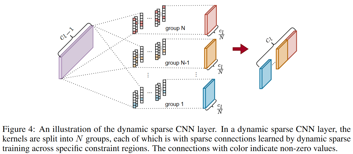
Following the main idea of the DST method, the proposed DSN model is trained sparsely from scratch to keep the kernel sparse. By design, the total number of activated weights must not exceed Nl ( 1 - S) during the training phase. However, we observe here that it is difficult to capture small eNRFs with the layer-wise search DST method, which finds the activated weights layer by layer, especially when the sparsity ratio S is small. Based on this observation, the kernels of each dynamics-parsed CNN layer are divided into different groups and their corresponding search regions are of different sizes, as shown in Fig. 4. contrary to the DST method, in DSN, the search for activated weights is done separately in different kernel groups, which is a more fine-grained strategy. Specifically, the kernel weights Θl ∈Rcl-1×cl×1×k in layer l are divided into N groups along the output channel. That is, 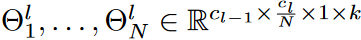 and the corresponding search region
  . The search region
  for the ith group in layer l is defined as the first
  positions of each kernel in this group. taking k=6 and N=3 as an example, the activated weights in the first group are only in the first two positions of each kernel in
  , while in the last group, they are in the whole kernel (as shown in Fig. 4 as shown). In this way, the various eNRFs can be covered, reducing the search space and improving search efficiency.
Given a weight search region  and a sparsity ratio S, we train the proposed DSN model as shown in Algorithm 1 (see original paper). The activated weights are explored in the search region and updated at each ∆t iteration. The ratio of updated weights decays over time according to the function fdecay (t; α, T) of the cosine annealing, as follows

where α is the initial percentage of updated activated weights, t is the current training iteration, and T is the number of training iterations. Thus, during the tth iteration, the number of updated activated weights in the i-th group of the l-th layer is  n, where
  is the number of weights that can be explored in the region
  . During the update of the activated weights, we first prune the activated weights determined at
  , followed by randomly generating new activated weights at
  . Here ArgTopK(v,u) gives the index of the top u elements with the highest value in vector v, RandomK(v,u) outputs the index of a random u element in vector v, and
  indicates the weights in
  except
  .
.
Searching for activated weights is straightforward. First, it is intuitive to prune weights that are small in magnitude. First, it is intuitive to prune small weights, since their contribution is insignificant or negligible. Also, considering the resilience of pruning, we can randomly regenerate the same number of new weights as the pruned weights to achieve a better search for activation weights. Thus, the search for weights is dynamic and plastic compared to the method of pruning weights before and after learning.
experiment
data-set
Details of each dataset are as follows
- Univariate TS datasets in the UCR 85 archive: This archive consists of 85 univariate TS datasets collected from various domains (e.g., health monitoring and remote sensing), with characteristic characteristics and varying levels of complexity. The number of instances in the training set ranges from 16 to 8926 and the time step resolution from 24 to 2709.
- Three multivariate TS datasets from UCI: The EEG2 dataset contains 1200 instances with 2 categories and 64 variables. The Daily Sport dataset contains 19 categories, 9,120 instances, and 45 variables.
Experimental setup and implementation details
Adam optimizer was used for optimization, with an initial learning rate of 3 × 10⁻⁴ and cosine decay of 10-4. 1,000 epochs were trained with a mini-batch size of 16. The number of kernel groups, N, was set to 3 to help cover small, medium, and large eNRFs. Each setting is repeated 5 times and the average result is reported.
Results and Analysis
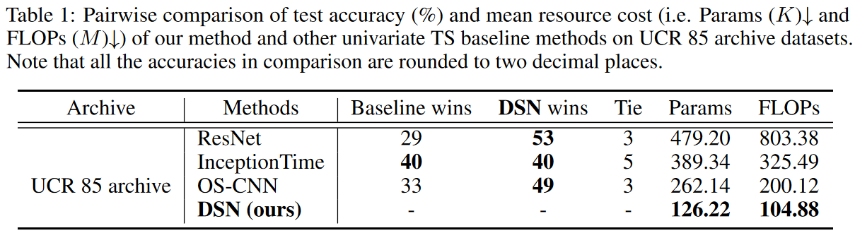
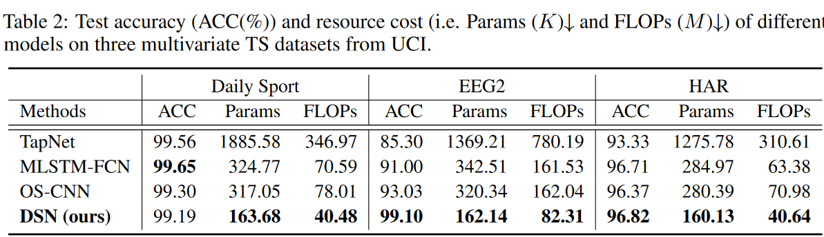
The performance on univariate and multivariate TSC benchmarks is shown in Table 1-2. For univariate TSC, we see that the proposed method outperforms the baseline method in most cases on the UCR 85 archive dataset with a smaller number of parameters (e.g. Params 3) and lower computational cost (e.g. FLOPs). For multivariate TSC, the proposed DSN method achieves better performance on EEG2 and HAR datasets, and MLSTM-FCN is 0.46% more accurate on Daily Sport. The resource cost (Params and FLOPs) of the proposed DSN is much smaller than the resource cost of the baseline method.
sensitivity analysis (e.g. in simulations)
Effect of sparse ratio
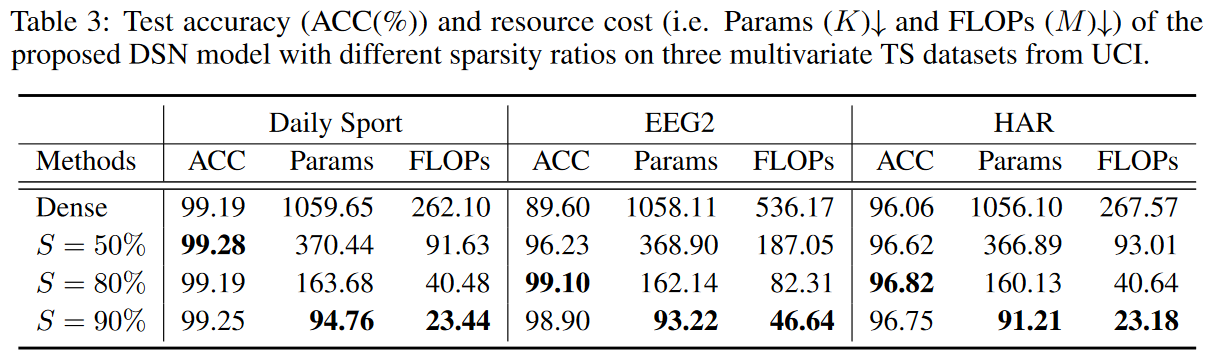
From Table 3, we can see how the sparsity ratio of the dynamic sparse CNN layer affects the final test accuracy and resource cost on the multivariate TS dataset. Here we analyze the trade-off between test accuracy and resource cost under various sparsity ratios (S ∈ [50%, 80%, 90%]) and dense DSN models. Note that a dense model is defined exactly like a DSN model where the entire kernel is densely connected. We find that more parameters in the model do not necessarily improve performance. This is mainly because increasing the number of parameters leads to overfitting, and with the right sparsity ratio, the desired receptive fields can be easily covered. This dataset is expected to have features from small receptive fields. Experiments show that sparsity of 80% reflects a good trade-off between accuracy and resource cost, which is the default setting for the dynamic sparse CNN layer of the DSN model here.
Architectural Effects
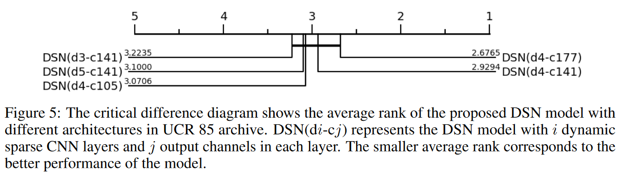
To show how the DSN architecture affects the final performance, a detailed comparison is made by employing the critical difference diagram that is usually used to evaluate TSCs; from Fig. 5, the DSN model with four dynamic sparse CNN layers and 177 output channels in each layer is consistently better than the other structures performance than the other structures. The proposed model with more output channels seems to be important to maintain the capacity of the network but requires more parameters and FLOPs compared to the other models. This highlights an interesting tradeoff between accuracy and computational efficiency. Experiments show that the DSN model with 4 dynamic sparse CNN layers and 141 output channels in each layer is a tradeoff between performance and resource cost, which is the default setting for the DSN model here.
Kernel Group Effectiveness
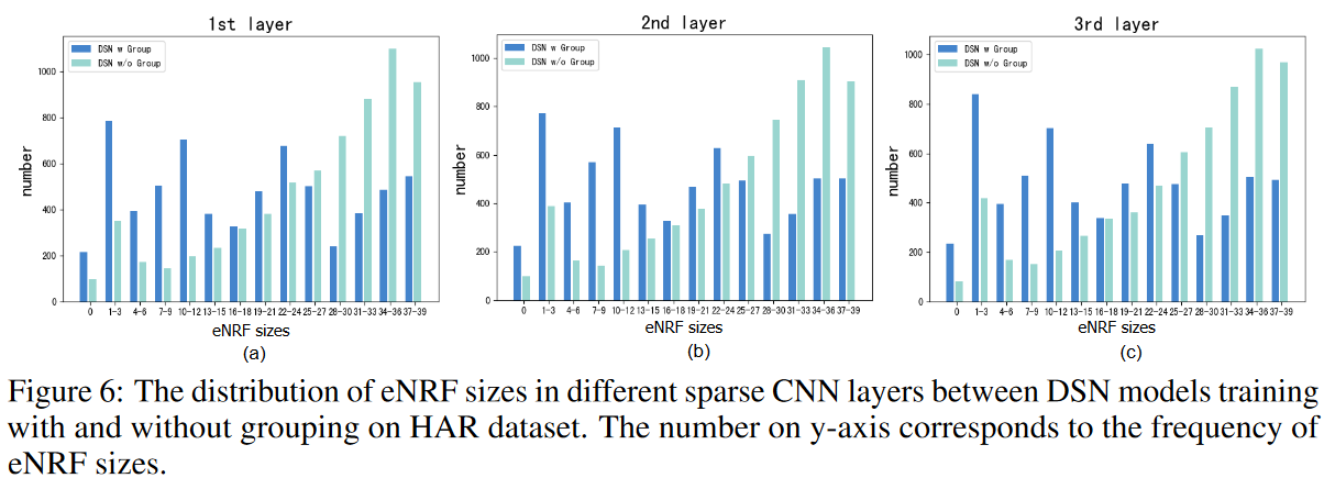
As shown in Fig. 6, training DSN without kernel groups hinders the capture of small eNRFs and cannot guarantee satisfactory performance on data sets such as EEG2, where local information is expected. The phenomenon of large RFs accounting for the majority of the training becomes more severe when the sparsity ratio S is reduced, and as shown in Table 4, the performance difference between training with groups and training without groups is large. By grouping the kernels, various RF coverage and advertising accuracies can be achieved on all datasets.

selective research
Effectiveness of Dynamic Sparse Training
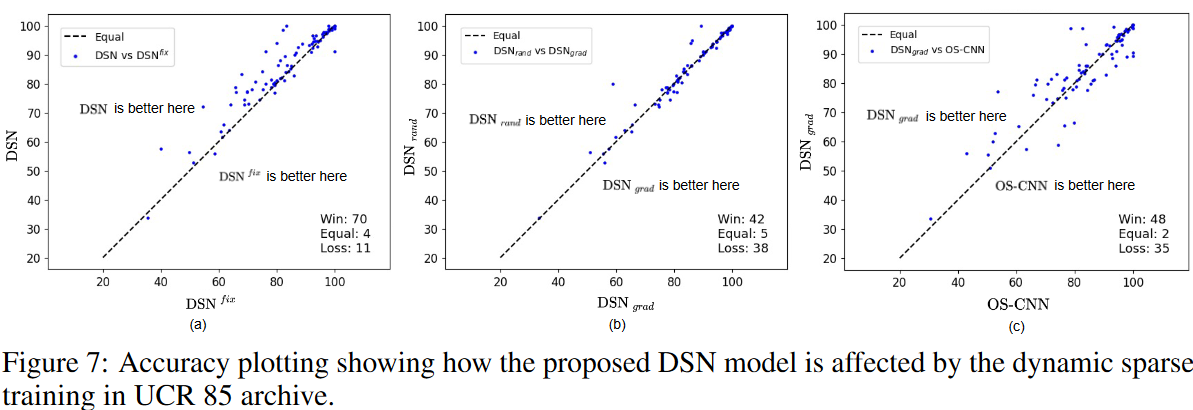
We also study the effect of dynamic sparse training on the DSN method: an ablation study was conducted to compare DSN with a static variant that fixes the topology during training after initialization of the activated weights (i.e., DSNfix). That is, the indicator function Il ( -) in Eq. (1) is not updated during training; the results shown in Fig. 7(a) indicate that the DSN model almost outperforms DSNfix in the UCR 85 archive and that what is learned by dynamic sparse learning are the appropriate activation weights and their values The results shown in (a) are as follows.
Case studies in other DST methods
Similarly, we analyzed the effectiveness of the proposed DSN method in the presence of other DST methods such as RigL, which grows weights with the largest gradient rather than randomly; from Fig. 7(c), we see that growing weights according to gradient (i.e. DSNgrad) can outperform the OS-CNN method in most cases of the UCR 85 archive. Furthermore, as shown in Fig. 7 (b), DSNgrad performs as well as the method of growing weights randomly (i.e., DSNrand). Note that DSNrand is the main setting for the method proposed in this paper because it does not require computing the full gradient at any given time. In summary, the proposed DSN with its fine-grained sparsity strategy can be easily combined with existing DST methods and shows potential for further improvement by integrating it with other advanced DST methods in the future.
Visualization of activation weights
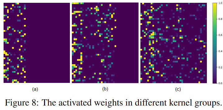
Fig. 8 shows the normalized activated weights of the DSN model after sparse training on the HAR dataset. (a), (b), and (c) correspond to the activated weights of the three kernel groups of the first dynamic sparse CNN layer, and each row in the figure represents one kernel. We see that the weights of each kernel are sparse and can be activated within the constraint region defined previously.
summary
This paper proposes a dynamic sparse network (DSN) for time series classification (TSC) that can learn to accommodate various receptive field (RF) sizes without the need for hyperparameter tuning. the DSN model, on both univariate and multivariate TSC data sets, state-of-the-art performance at less computational cost than recent baseline methods. The proposed DSN model provides a viable solution to bridge the gap between resource awareness and effective adjacent receptive field coverage of a variety of TSCs and has the potential to inspire other researchers in a variety of fields.


Categories related to this article


