Volatility Prediction With GARCH!
3 main points
✔️ Volatility forecasting using GARCH
✔️ Volatility forecasting for 10 stocks listed on the National Stock Exchange (NSE) of India
✔️ Asymmetric GARCH model is more accurate than the symmetric GARCH model
Volatility Modeling of Stocks from Selected Sectors of the Indian Economy Using GARCH
written by Jaydip Sen, Sidra Mehtab, Abhishek Dutta
(Submitted on 28 May 2021)
Comments: Accepted at IEEE ASIANCON'2021.
Subjects: Computational Finance (q-fin.CP); Machine Learning (cs.LG); Statistical Finance (q-fin.ST)
code:
The images used in this article are from the paper, the introductory slides, or were created based on them.
such as ...
Volatility clusters are important characteristics that have a significant impact on the behavior of the stock market.
In this paper, we present several volatility models based on the generalized autoregressive conditional heteroskedasticity (GARCH) framework to model the volatility of ten stocks listed on the National Stock Exchange (NSE) of India.
The stocks are selected from the automobile and banking sectors of the Indian economy and have a significant impact on the sectoral indices of each sector on the NSE. This paper presents a series of volatility models based on the Generalized Autoregressive Conditional Heteroskedasticity (GARCH) approach.
We select the top five stocks from each of the two important sectors of the Indian economy, the automobile sector and the banking sector, and build a model using historical stock price data from the NSE from January 1, 2010 to April 30, 2021. After building and fine-tuning several GARCH models, we back-test them with out-of-sample data.
There are two features of this study.
The first proposes a series of GARCH models that have been constructed, fine-tuned and back-tested using over a decade of real-world stock price data for various sectors of the Indian stock market.
Secondly, we provide a benchmark to compare the volatility of the two sectors studied in this research.
By getting the volatility of the two sectors right, potential investors can understand the associated risks and returns of the sectors.
Related research
Quite a few models based on the GARCH (1,1) framework have been proposed, and it has been observed that the generalized distribution of residuals in these models is more accurate in assessing the volatility of a series than other models of residuals . Some studies have found that the asymmetric GJR-GARCH model produces more accurate predictions about the conditional variance when volatility is high, but in the real world mostly, the EGARCH model produces more accurate predictions in situations of asymmetric volatility.
It has been observed that GARCH based volatility models yield more stable and robust forecasts while the sensitivity of entropy based forecasts is higher. The return analysis of 15 important sectors of Indian economy is based on the predictive output of deep learning based LSTM network model.
The study reveals that the FMCG sector remains the most profitable sector, but the power sector has the lowest aggregate returns. A multivariate GARCH model is also proposed to analyze the volatility of several contemporaneous time series.
Data and Methodology
The methodology followed in this study consists of ten steps. In the following, each step is explained in detail.
data extraction
Extract stock price data from the Yahoo Finance website using the panadas module's DataReader API.
For example, if we want to extract the share price records of Maruti Suzuki listed on NSE from Yahoo Finance website from start date to end date with the attributes of high, low, open, close, volume and adjusted close, the python code required is as follows maruti = web.DataReader ('MARUTI.NS', 'yahoo', start, end)[['High', 'Low', 'Open', 'Close', 'Adj Close']]. For all issues, the start date is January 1, 2010, and the end date is April 30, 2021.
Calculation of Hurst Index and Volatility
After extracting the stock price records, the Hurst index of the time series of closing prices is calculated. The Hurst index is a measure of the long-run behavior of a time series. It measures the autocorrelation between the different lag values of the time series and calculates the rate at which the autocorrelation decreases with the lag value. Based on these calculations, the Hurst index calculates a measure that determines if the time series is strongly regressing to the mean or if it is clustering in an upward to downward direction. Here, we calculate the Hurst index for all stocks using a function that calculates autocorrelation with up to 100 lags.
After calculating the Hurst index of a stock based on the closing index of the stock, the volatility of the series is calculated.
Daily volatility is determined by calculating the standard deviation of the daily return values. Monthly and annual volatilities are calculated by multiplying the daily volatility by a factor of the square root of 21 and the square root of 252, respectively, assuming that there are 21 business days in a month and 252 business days in a year.
Investigation of statistical properties of return series and log return series
In this step, the return series and log return series are calculated.
To calculate the return series, we use Python's pct_change function. The log return series is calculated by first applying the log function to the closing prices of the stocks: the return series, the log return series, their quantile-quantile (Q-Q) plots, autocorrelation function (ACF) plots, and partial autocorrelation function (PACF) plots.
Fitting a GARCH(1,1) model with constant mean and normally distributed residuals
In this step, we construct a volatility model for a time series of stock prices. First, we construct a GARCH(1,1) with a constant mean and normally distributed residuals. This type of GARCH model can be represented as in (1).
The first term, ω, represents the constant variance corresponding to the long-run average volatility, the coefficient α represents the effect of squaring the residual value at time t-1, and the coefficient β represents the effect of the variance at time t-1 on the volatility at time t.
![]()
In the GARCH model, we use the residuals as volatility shocks (sudden changes). In the GARCH (1,1) model in this step, we assume that the residuals follow a normal distribution with zero mean. The residuals at time t are given by (2).
(2), which represents the return at time instant t and is the average of the return series.
![]()
We fit a GARCH (1,1) model with a constant mean and normally distributed residuals. We determine the values of the parameters ω, α, and β of the GARCH model and their respective p-values. We also find the Akaike Information Criterion (AIC) of the model.
The Akaike Information Criterion... A statistic that evaluates the predictive quality of a statistical model using the difference between observed and theoretical values (residuals). The smaller the value, the better the fit.
Fitting a GARCH(1,1) model with constant mean and skewed t-distribution of residuals
Since the values of stock return and log return usually do not follow a normal distribution, we assume that the residuals follow a skewed t-distribution rather than a normal distribution and fine-tune the GARCH model constructed in step 4.
We also tested how accurate the GARCH(1,1) model is by plotting the volatility of the skew-t error distribution against the daily returns of the GARCH(1,1) model.
Identifying the optimal ARMA model for log return series
In this step, we find the autoregressive moving average (ARMA) model that best fits the logarithmic return series of stock prices.
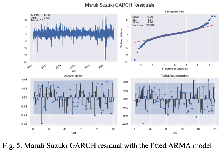
Create a fitting model for ARMA residuals to GARCH(1,1)
An optimal ARMA model is fitted to the log return series and a GARCH (1,1) model that is fitted to the series and has a zero mean (because the residuals are assumed to have a zero mean) is fitted to the residuals of the ARMA model.
Using the summary function of the GARCH model, we find the parameters ω, α, β and their corresponding p-values. The AIC of the model is also noted; the significance level of the p-value indicates the goodness of fit of the model.
Fit an asymmetric volatility model to the return series and evaluate the fit of the model
The GARCH model constructed in the previous step assumes that positive and negative news have a similar impact on volatility. This assumption does not hold in the real world, where the impact of negative news on return volatility is greater than the impact of positive news.
In order to effectively model the volatility of the return series, the GARCH model must have the ability to handle asymmetries in the effects.
For this purpose, we construct two asymmetric models, (i) GJR-GARCH and (ii) EGARCH.
The GJR-GARCH(1,1,1) model is given by (3). In (3), γ is an asymmetric parameter and d_(t-1) is a dummy variable. If the residual of the previous time is negative, the value of the dummy variable is 1, and if the residual of the previous time is positive, the value of the dummy variable is 0.
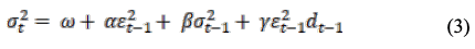
The EGARCH(1,1,1) model is given as (4)
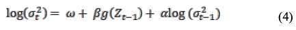
In (4), we evaluate the value of the function as follows
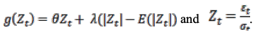
For θ = 0, the larger the shock, the larger the conditional variance. If (Z_t - E[Z_t]>0), the conditional variance decreases.
Also, if the shock is smaller than the mean, the shock to variance will be positive We plot the predicted volatility values of the GJR-GARCH and EGARCH models against the return series to see how close the predicted volatility values are to the actual volatility values of the return series.
EGARCH Validating the accuracy of volatility forecasts
This step uses two different forecasting methods, the expanding window method and the fixed window method, to compute the forecasts. In this step, we calculate the forecasted volatility by the EGARCH model for out-of-sample data from January 1, 2021 to April 30, 2021 using two different forecasting methods, the expanding window method and the fixed window method. The results are as follows.
In the fixed window method, the volatility value for the next 5 days is predicted based on the volatility of the previous 5 days. In the expanding window method, the size of the training window increases with the number of rounds of forecasting. Finally, we plot the predicted volatility values and the predicted and actual volatility values of the volatility.
Backtesting the EGARCH model with out-of-sample data
In the last step, we backtest the EGARCH model against the return series. We backtest the EGARCH model against the return series and calculate the mean absolute error (MAE).
experimental results
We present extensive experimental results on the performance of various GARCH-based volatility models.
Automotive Sector
Top 5 stocks in Automobile Sector listed on NSE The top 5 stocks in Automobile Sector listed on NSE are Maruti Suzuki India (MSZ), Mahindra and Mahindra (MAH), Tata Motors (TAM), Mahindra and Mahindra (MAH).and Mahindra (MAH), (iii) Tata Motors (TAM), (iv) Bajaj Auto (BAJ) and Hero Motocorp (HMC). The percentage weightage of each of these five stocks used to calculate the respective Auto Sector Index of these five companies is as follows: msu-18.72, mmh-15.72, tmo-11.50, baj-10.89, hmc-7.99.
Only the visuals of the topmost stocks in each sector are shown in Table I. Figure 1 also shows the key features of the logr return series for Maruti Suzuki stocks.
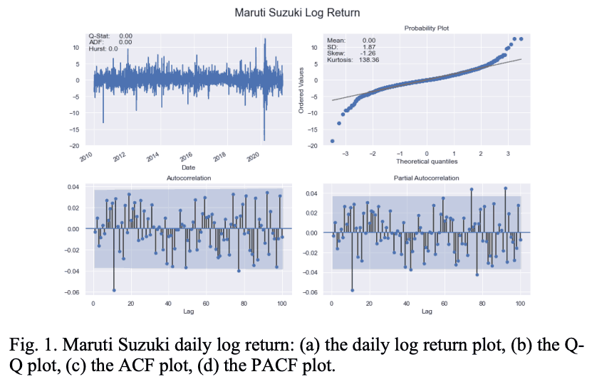
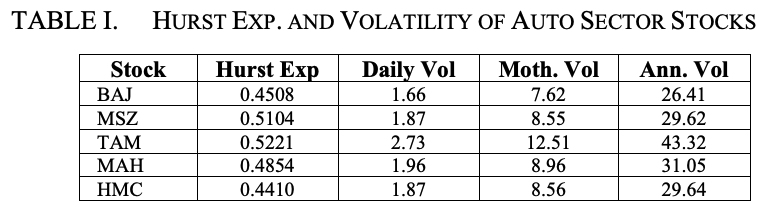
Figure 2 illustrates the characteristics of the daily volatility series for Maruti Suzuki.
Table I shows that the BAJ, MAH, and HMC stocks From Table 1, the BAJ, MAH, and HMC stocks exhibit mean reversion characteristics, while the MSZ and TAM series exhibit mild mean reversion characteristics in terms of the Hurst index.
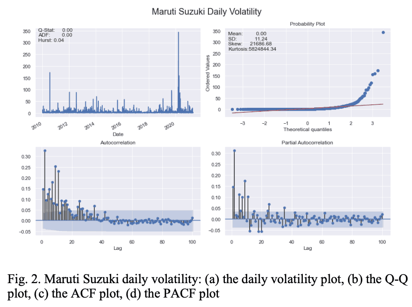
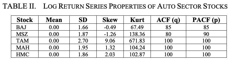
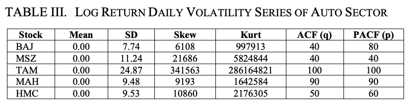
Table II and Table III show the log return series of the auto sector stocks and the important statistical properties of the daily volatility of the log return series. From Table II, it is clear that the mean value of the log return series for all stocks is zero, but the standard deviation, skewness, and kurtosis of the TAM are the highest.
The same observation is noted in Table III.
Therefore, we can conclude that TAM is the most volatile stock in the automotive sector. On the other hand, BAJ is found to exhibit the lowest volatility in the sector.
Both the ACF and PACF plots of the daily log return series and the daily volatility series are found to be significant at large values of lag; when the ACF and PACF plots are plotted against the maximum value of lag, 100, these plots are found to be significant at large lags It was found that.
Next, we fit the GARCH(1,1) model to the return series with the mean constant, the volatility model as GARCH, and the error distribution as normal. Table IV shows the results of fitting the GARCH(1,1) model to the return series of five stocks in the automotive sector. The columns in Table IV show, respectively, the name of the stock (Stock), the number of iterations required to fit the model to the data of the return series (#Iterations), the number of evaluations of the function (i.e., the log-likelihood function) (Func Eval), the number of updates of the gradient (Grad Eval), and the value of the log-likelihood function (Log-Likelihood) of the log-likelihood function.
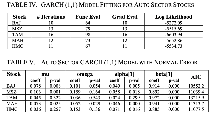
Table V gives an overview of the GARCH (1,1) model with a constant mean and normally distributed errors.
The parameter mu means constant mean, omega means constant variance corresponding to the long-run average volatility, alpha means new information in this round that was not available in the previous round, and beta means the predicted volatility in the previous period.
The larger the value of alpha, the greater the impact of the shock. On the other hand, the larger the value of beta, the longer the duration of the shock.
In Table V, we observe that the alpha is highest in MSZ and lowest in TAM. Thus, the impact of shocks is highest in MSZ and lowest in TAM stocks. On the other hand, based on beta values, the duration of shocks is found to be the longest for TAM and the shortest for HMC.
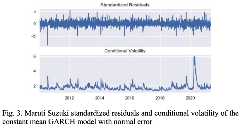
Figure 3 shows the pattern of standardized residuals and conditional volatilities of MSZ stocks computed with the GARCH(1,1) model assuming constant mean and normally distributed residuals.
Next, we change the error model from normal to skewed. In financial time series, the residuals are almost always not normally distributed, so the assumption that the residuals follow a skewed t-distribution is more realistic than the assumption that they follow a skewed t-distribution.
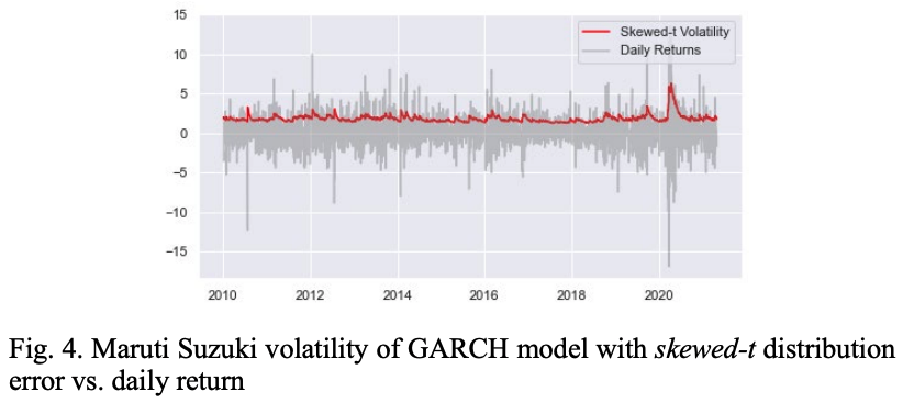
Figure 4 compares the volatility of the GARCH model with residuals from the skewed-t distribution with the daily return values of MSZ stocks.
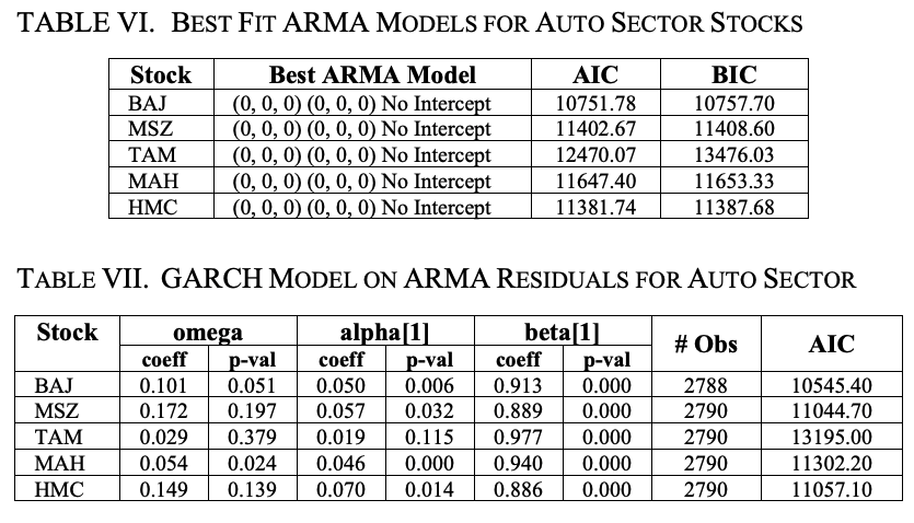
To further refine the GARCH(1,1) model, we model the log return of the stock's closing price with an ARMA model, fit the residuals of the ARMA model, and estimate the volatility of the log return series with a new GARCH model.
Table VI shows the results; it can be seen that for all five stocks, the ARMA (0,0,0) (0,0,0) without intercept is the best fitting model. The residuals of this ARMA are fitted to a zero-mean GARCH (1,1) model.
Table VII shows the results for five stocks.
To further improve the accuracy of the GARCH model, two asymmetric models are constructed using the concepts of GJR-GARCH and EGARCH. First, we fit the GJR-GARCH model to the return series of automotive sector stocks. The mean is constant, the residuals are t-distributed, and the volatility is an asymmetric GARCH pattern.
The asymmetric shocks considered in this model are of one lag. Table VIII provides a summary of the model for five stocks in the auto sector. It can be seen that almost all of the gamma and beta coefficients are significant.
It was found to be the most important predictor in the GJR-GARCH volatility model for the automotive sector.
Finally, we construct another asymmetric volatility model using EGARCH(1,1,1). Unlike the other GARCH models, EGARCH does not require the alpha and beta parameters to be non-negative. Hence, less time is required to construct the EGARCH model. Table IX gives an overview of the EGARCH model for stocks in the automotive sector. It can be seen that the model fits the return values of the stocks very well as almost all the coefficients of alpha, gamma and beta are significant.
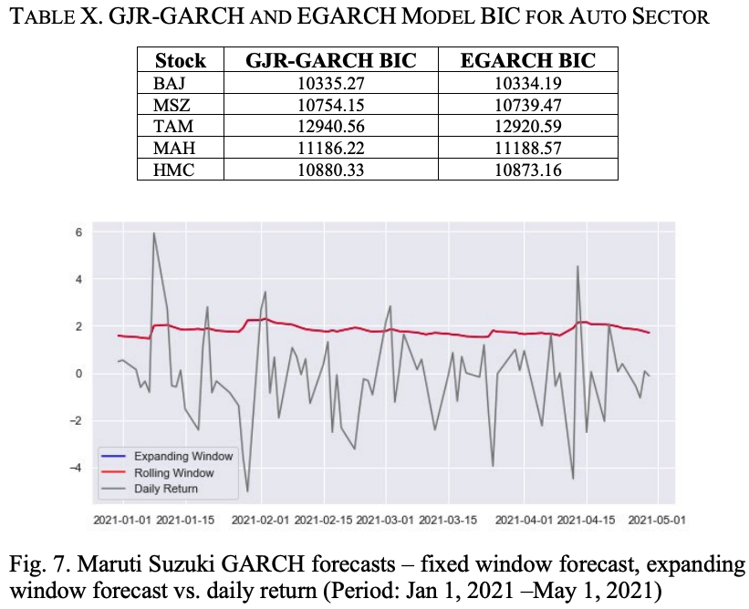
Table X shows the BIC values of the GJR-GARCH and EGARCH models for the automotive sector stocks; except for MAH, we find that the BIC of the EGARCH model is lower than the BIC of the corresponding GJR-GARCH model. Figure 6 shows the MSZ return series, the GJR-GARCH volatility, and the EGARCH volatility. We can see that the performance of both GARCH models is almost the same and both models accurately capture the volatility of the MSZ return series.
Using the expanded rolling window method and the fixed rolling window method, we predicted the volatility of the MSZ return series from January 1, 2021, using 80 data points. The results are shown in Figure 7. We can see that both forecasting methods produce the same forecasting results.
To evaluate the performance of the EGARCH model against the return series of the automotive sector stocks, we back-tested the model.
Table XI shows the mean absolute error (MAE) and root mean square error (RMSE) of the model for the five stocks. The high values of MAE and RMSE for TAM are attributed to the high volatility of the stock.
Banking Sector.
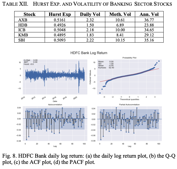
The five stocks that contribute the most to the calculation of the NSE Banking Sector Index and their respective weights (%) are as follows. (i) HDFC Bank (HDB)-27.41, (ii) ICICI Bank (ICB)-21.09, Axis Bank (AXB)-14.30, Kotak Mahindra Bank (KMB)-13.02 and State Bank of India (SBI)-11.74. Table XII shows the Hurst index, daily, monthly and annual volatility of five stocks of the banking sector. It can be seen that AXB, ICB, and SBI show very mild trendiness while HDB and KMB are mean reverting; AXB is the most volatile stock while HDB is the least volatile stock among the five stocks.
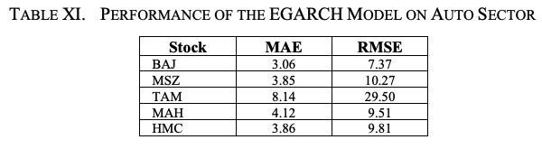
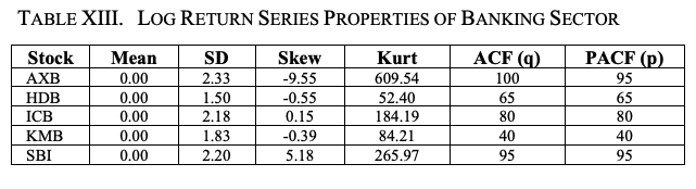
Table XIII and Figure 8 show the key statistical properties of the log return series for banking sector stocks. Although the mean of all return series is zero, we find that the SD of AXB is the largest. Also, the magnitude of skewness and kurtosis of AXB is the highest among the five banking sector stocks, indicating that AXB is the most volatile among the banking sector stocks.
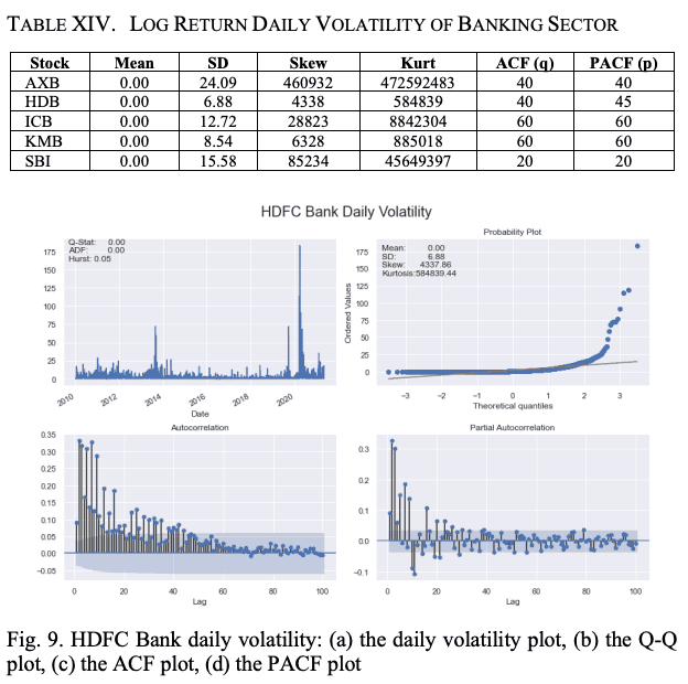
We use a maximum lag value of 100 for the ACF and PACF plots. Table XIV and Figure 9 show the volatility characteristics of the log return series for each stock. Again, we see that the mean values of the daily log return volatilities are all zero; AXB has the highest SD, skewness, and kurtosis values of the log return series volatilities.
As in the case of automotive sector stocks, we fit a constant mean GARCH(1,1) model to the return series and normally distribute the residuals.
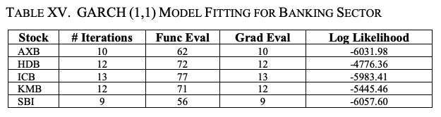
Table XV presents the results of the model fitting for five stocks in the banking sector. The meaning of the column names in Table XV is the same as the column names in Table IV discussed earlier.
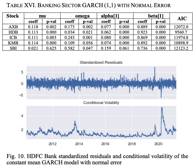
A summary of the constant mean GARCH(1,1) model with normally distributed residuals for banking sector stocks is shown in Table XVI. As explained earlier, the parameters mu, omega, alpha, and beta stand for constant mean, long-run constant variance, coefficient of the square of the residual value in the last round, and coefficient of the variance of the volatility forecast in the last round.
The higher the alpha value, the greater the impact of the shock on volatility, and the higher the beta value, the longer the impact is valid. We find that SBI has the highest alpha value and HDB has the lowest parameter value. It is the lowest for HDB. Thus, the impact of shocks is the highest for SBI and the lowest for HDB. Looking at the beta values, HDB has the longest period affected by shocks and SBI has the shortest period affected by shocks.
The standardized residuals and conditional volatilities of the HDB stock return series calculated by the GARCH(1,1) model are shown in Figure 10. This GARCH model is constructed based on two assumptions.
(i)The mean value of the return series is constant.
(ii)The residuals are normally distributed.
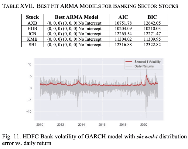
To make the model more realistic, as we did with the auto sector stocks, we build the GARCH model with the assumption that the residuals follow a skewed t-distribution instead of a normal distribution. Figure 11 shows the volatility of the GARCH model with skewed t-distribution residuals and the daily return values of HDB stocks.
Next, we fine-tune the GARCH(1,1) model.
Construct an ARMA model using the log return of the stock's closing price; fit the residuals of the ARMA model to a GARCH model and estimate the long-term volatility of the log return series. We fit the ARMA model to the log return series of stocks. Table XVII shows the results. We find that for all the five stocks in the banking sector as well as the stocks in the automobile sector, ARMA (0,0,0) (0,0,0) with no intercept is the best fitting model; a zero-mean GARCH (1,1) model is fitted to the residuals of the ARMA model.
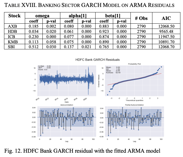
A summary of the GARCH model is shown in Table XVIII, where most of the coefficients of ω, α, and β show significant p-values, indicating that the fit of the model is very good. As in the case of auto sector stocks, we construct two asymmetric models, EJR-GARCH and EGARCH, to make the volatility model more accurate.
First, we construct a GJR-GARCH model. A constant-mean GJR-GARCH model is created, and the residuals follow a t-distribution, with asymmetric shocks of one lag being significant.
An overview of this model is given in Table XIX.
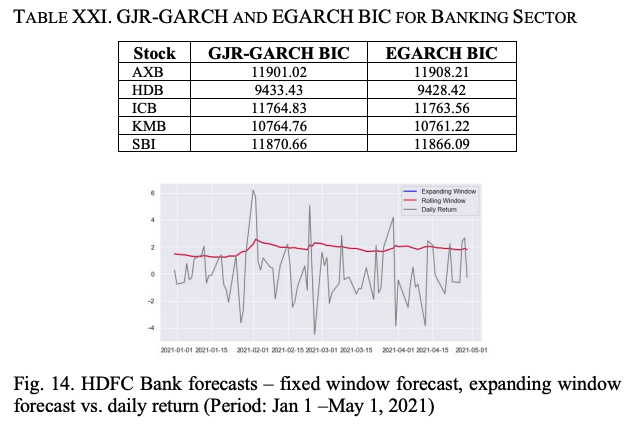
Since all gamma and beta coefficients are significant, it is clear that the one-lag asymmetric shocks and the one-lag variance are the main components of the model. The results for the EGARCH(1,1) model in Table XX show that the model is a better fit than the GJR-GARCH(1,1) model as all coefficients are significant. From Table XXI, it is clear that the BIC of the EGARCH model is smaller than the BIC of GJR-GARCH for all the stocks except AXB, indicating a better fit to the stock price data.
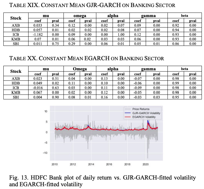
Figure 14 shows the HDB return series and the volatility of GJR-GARCH and EGARCH.
Table XXII shows the mean absolute error (MAE) and root mean square error (RMSE) of the EGARH model for all the five stocks in the banking sector. It can be seen that the model performs very well for out-of-sample data.
 Finally.
In this paper, we have proposed several volatility models based on different variants of GARCH. These models are constructed based on historical stock price data from January 1, 2010, to April 30, 2021.
2021. stocks were selected from the automobile and banking sectors of the Indian NSE. After fine-tuning the model, we back-tested it with out-of-sample data to assess its accuracy in predicting the future volatility of stocks. It was observed that the asymmetric GARCH model outperformed the symmetric model, but EGARCH was found to give the most accurate results.


Categories related to this article
.JPG)


