
Time Series Anomaly Detection With Model Selection By Reinforcement Learning
3 main points
✔️ There are several patterns of time series anomaly, and models that specialize in one pattern may not be good at detecting other patterns of anomaly.
✔️ This method RLMSAD tackles this problem. It pools models (5 in this case) that detect dissimilar patterns with different features and use reinforcement learning to select which model is appropriate for a particular time-series data.
✔️ We have confirmed that this method outperforms traditional models.
Time Series Anomaly Detection via Reinforcement Learning-Based Model Selection
written by Jiuqi Elise Zhang, Di Wu, Benoit Boulet
(Submitted on 19 May 2022 (v1), last revised 27 Jul 2022 (this version, v4))
Comments: Accepted by IEEE Canadian Conference on Electrical and Computer Engineering (CCECE) 2022
Subjects: Machine Learning (cs.LG)
code:

The images used in this article are from the paper, the introductory slides, or were created based on them.
outline
Time series anomaly detection is very important for the reliable and efficient operation of real-world systems. Many anomaly detection methods have been developed based on various assumptions about the characteristics of the anomaly. However, due to the complexity of real-world data, different anomalies in a time series usually have diverse aspects that require different anomaly assumptions. This makes it difficult for a single anomaly detector to outperform all models at all times. To exploit the advantages of different base models, we propose a model selection framework based on reinforcement learning. Specifically, we first learn a pool of different anomaly detection models and then use reinforcement learning to dynamically select candidate models from these base models. Experimental results on real-world data demonstrate that the proposed method outperforms all models in terms of overall performance.
first of all
Smart Grid, as a part of cyber-physical systems technology, aims to improve the safety and efficiency of the power grid by utilizing advanced infrastructure, communication networks, and computational techniques. The Smart Grid is used as the evaluation environment for this thesis.
An outlier is defined as "an observation that appears to be inconsistent with the rest of the set. Alternatively, they are defined as "data points that deviate from the pattern or distribution of the majority of the data columns" or data points that are out of the distribution. The occurrence of such anomalies usually indicates a potential risk in the system. For example, anomalous meter readings in the power grid may indicate a failure or a potential cyber attack, while anomalies in a financial time series may indicate "fraud, risk, identity theft, network intrusions, account takeover, money laundering or other illegal activities". Anomaly detection is therefore important to ensure the operational safety of systems and is finding applications in areas such as medical systems, online social networks, the Internet of Things (IoT), and smart grids.
An anomaly detection device is usually built on one of the following assumptions
(1) Variations occur with low frequency.
Under this assumption, anomalies are most likely to occur in regions of low probability or at the tail of the distribution if the underlying probability distribution of the data can be characterized. One study on anomaly detection in data streams fits the extreme value distribution of the input data stream based on Extreme Value Theory (EVT) and utilizes the PeaksOverThreshold (POT) approach to estimate normality bounds for anomaly detection. In another study on anomaly detection in power system metering ], the authors propose to approximate the probability distribution of meter measurements using kernel density estimation (KDE) and further propose a probabilistic autoencoder to reconstruct the upper and lower bounds of the statistical interval for normal data.
(2) Anomalous instances are most likely to occur far away from the majority of data or in areas of low density
Methods based on this assumption often incorporate the concept of nearest neighbors and data-specific distance/proximity/density metrics. In one recent study, the detection performance of the k-Nearest Neighbors (kNN) algorithm was compared to several state-of-the-art deep learning-based self-supervised frameworks, and the authors found that the simple nearest neighbor-based approach still outperformed them. In one study on anomaly detection in the Internet of Things (IoT), the authors propose a Local Outlier Factor (LOF) hyperparameter tuning scheme.
(3) If a good representation of the input dataset can be learned, anomalies are expected to have significantly different profiles than normal instances. Alternatively, if further future data is reconstructed or predicted from the learned representation, the reconstruction based on the anomaly is expected to be significantly different from the reconstruction based on normal data.
In a recent study, the authors have proposed an anomaly detection framework OmniAnomaly consisting of GRU-RNN, Planar Normalizing Flows (Planar NF), and Variational Autoencoder (VAE) for learning and reconstructing the data representation The proposed framework is based on the following two steps. The reconstruction probability under a given latent variable is then used as the anomaly score. In another study on spacecraft anomaly detection, a non-parametric thresholding scheme is proposed to predict the future value of a sequence using LSTM-RNN and to interpret the prediction error. A large prediction error means that there is a high probability of anomalies in the time series.
However, due to the complexity of real-world data, anomalies can appear in many different forms. During the testing phase, anomaly detectors based on certain assumptions about anomalies tend to favor certain aspects over others. That is, a single model may be sensitive to certain types of anomalies while tending to overlook others. There is no universal model that outperforms all other models for different types of input data.
To exploit the advantages of multiple basic models at different time phases, we propose to dynamically select the best detector from a pool of candidate models at each time phase. In the proposed setup, the current anomaly prediction is based on the output of the currently selected model. Reinforcement learning (RL) seems to be a logical solution to this challenge as a machine learning paradigm concerned with "mapping situations into actions by maximizing the numerical reward signal". Reinforcement learning agents aim to learn optimal decision-making policies by maximizing the total reward. Reinforcement learning has been applied to a variety of real-world problems such as electric vehicle charging scheduling, home energy management, and traffic signal control. The effectiveness of dynamic model selection has also been demonstrated in various areas such as model selection for short-term load forecasting, model combination for time series forecasting, and dynamic weighting of ensembles for time series forecasting.
We propose a model selection framework for anomaly detection based on reinforcement learning (RLMSAD). The objective of the proposed framework is to select the optimal detector at each time step based on the observed values of the input time series and the predictions of each base model. Experiments on a real-world dataset, Secure Water Treatment (SWaT), show that the proposed framework outperforms each base detector in terms of model accuracy.
technical background
Unsupervised anomaly detection in time series
A time series (X = {x1, x2, ..., xt}) is a sequence of data indexed by time. A time series can be univariate, where each xi is a scalar, or multivariate, where each xi is a vector. In this paper, we address the problem of anomaly detection in multivariate time series in an unsupervised setting. The training sequence Xtrain is a time series containing only normal instances, while the test sequence Xtest is contaminated with anomalous instances. In the training phase, an anomaly detector is pre-trained on Xtrain to capture the features of normal instances. In testing, the detector examines Xtest and outputs an anomaly score for each instance. By comparing this score to an empirical threshold, we obtain an anomaly label for each test instance.
Markov Decision Processes and Reinforcement Learning
Reinforcement Learning (RL) is one of the machine learning paradigms that deals with sequential decision-making problems.
It aims to train agents to discover the optimal behavior in the environment by maximizing the total reward and is usually modeled as a Markov decision process (MDP). A standard MDP is defined as a tuple, M = (S, A, P, R, γ). In this expression, S is the set of states, A is the set of actions, P(s'|s, a) is the matrix of state transition probabilities, and R(s, a) is the reward function. γ is the discount factor for the reward calculation, usually between 0 and 1. In a deterministic MDP, each action leads to a certain state, i.e., the dynamics of state transitions are fixed, so there is no need to consider the matrix P(s'|s, a), and the MDP can be expressed in turn by M = (S, A, R, γ). The return Gt
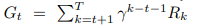
is the future cumulative reward after the current time stept. Also, policy π(a|s) is a probability distribution that maps the current state to the likelihood of choosing a particular action. The reinforcement learning agent aims to learn a decision policy π(a|s) that maximizes expected total returns.
technique
Overall workflow
The model workflow is shown in Fig. 1. The time series input is segmented in sliding windows. In each segmented window, the last timestamp is the instance to be analyzed and all previous timestamps are used as input features. Each candidate anomaly detector is first individually pre-trained on the training set. Then, all detectors are run against the test data and each detector computes a set of anomaly scores for all test instances. To interpret the anomaly scores, an empirical anomaly threshold must be determined for each base detector. Based on the scores and thresholds, every base detector can generate a set of predictive labels for the test data.
Using the prediction scores, empirical thresholds, and prediction labels obtained in the previous step, two more confidence scores are defined. These two confidence scores, together with the prediction scores, thresholds, and prediction labels, are integrated into a Markov Decision Process (MDP) as state variables; once the MDP is constructed, the model selection policy can be learned using an appropriate reinforcement learning algorithm (we use DQN in our implementation here).

Performance evaluation of base detector
To characterize the performance of candidate detectors in the model pool, we propose the following two scores. Each anomaly detector generates a set of anomaly scores for the test data. Typically, a higher anomaly score indicates a higher likelihood of an anomaly is present. Consequently, the higher the predicted score exceeds the model threshold, the more likely it is that the corresponding instance is anomalous under the current model prediction. Therefore, one might evaluate the validity of a model's predictions based on the extent to which a given score exceeds the threshold value. Here, we propose the Distance to-Threshold Confidence (DistancetoThresholdConfidence ).
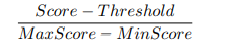
is computed by how much the current score exceeds the threshold value for the difference between the maximum and minimum score (scaled down to the range [0, 1] on the min-max scale). We also propose Prediction-Consensus Confidence, inspired by the idea of majority voting in ensemble learning.
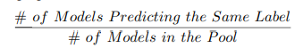
It is calculated as the number of models making the same prediction relative to the total number of candidate models. The more candidate models generate the same prediction in the pool, the more likely the current prediction is true.
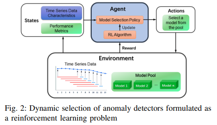
Markov Decision Process (MDP) Formulation
The model selection problem is formalized as a Markov decision process as follows (see Fig. 2). In this setting, the state transitions are deterministic because they naturally follow a time sequence as time steps in a sequence. That is, the state transition probability P(s'|s) is 1 for every pair of nearest consecutive states from st to st+1 and 0 otherwise. The discount factor γ is set to 1 (undiscounted).
- condition
The state space is the same size as the model pool. We consider each state as a selected anomaly detector, and the state variables include a scaled anomaly score, a scaled anomaly threshold, a binary prediction label (0 for normal, 1 for anomaly), a distance-threshold confidence level, and a prediction-agreement confidence level. Note that for each base detector, its anomaly score and threshold are normalized to [0, 1] using the min-max scale.
- action
The action space is discrete and has the same size as the model pool. Here, each action that selects one candidate detector from the pool is characterized by the index of the selected model in the pool.
- reward
The reward function is determined based on a comparison of the predicted and actual labels. This is denoted by (r1, r2, r3, r4 > 0).
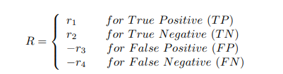
The rewards are designed to encourage the agent to make appropriate model choices in a dynamic environment. We view anomalies as "positive" and normal instances as "negative"; True positive (TP) represents a state where both the predicted and ground-truth labels are "abnormal" and the model correctly identifies anomalies; True negative (TN) represents a state where both the predicted and False positive (FP) represents the case where the predicted label is "anomalous" and the ground truth label is "normal" and the model correctly identifies normal instances. False negative (FN) represents a scenario where the predicted label is "normal" and the ground truth label is "abnormal", meaning that the model misses the anomaly and misclassifies it as normal. It means that the model misses the anomaly and misidentifies it as normal.
Given the real-world implications of the above four scenarios, we propose the following assumptions regarding reward setting. The majority of instances are normal and anomalies are relatively rare. Therefore, we consider that correctly identifying normal instances is a more trivial case. From this perspective, the reward for TN should be relatively small and the reward for TP should be relatively large, i.e. r1 > r2.
Ignoring actual anomalies is also generally more harmful than giving false alarms. Sometimes, it can encourage the model to be rather hypersensitive and "bold" with positive predictions. In this way, the model may generate more FPs, but also reduce the risk of ignoring actual anomalies. In this respect, the model is penalized more severely when it fails to detect an actual anomaly (in the case of FN), i.e. r4 > r3, than when it generates a false alarm (in the case of FP).
experiment
data-set
The dataset used for the evaluation is the Secure Water Treatment (SWaT) Dataset collected by iTrust, a cybersecurity research center at the Singapore University of Technology and Design. This dataset collects operational data from 51 sensors and actuators in an industrial water treatment testbed. The experiment here was conducted in the December 2015 version and includes 7 days of normal operation data and 4 days of data contaminated by an attack (outliers). This is a multivariate time series dataset with 51 features: the 7-day normal data contains 496,800 timestamps and has been selected as a pre-training set. The 4 days of data under attack contains 449,919 timestamps and is selected as the test set. The percentage of anomalous data in the test set is 11.98%.
base model
When forming the model pool, we ensure diversity of choice by selecting models based on different anomaly assumptions. The following five unsupervised anomaly detection algorithms are selected as candidate models
- One-Class SVM (One-Class SVM )
A method for novelty detection based on support vectors. The goal is to learn a hyperplane that separates regions of high data density from regions of low data density.
- Isolation Forest (iForest)
The Isolation Forest algorithm is based on the assumption that anomalies are easily isolated. If multiple datasets/dataset information/decision trees are fitted to a dataset, then anomalous data points should be more easily isolated from the majority of the data. Therefore, we would expect to find anomalies in leaves relatively close to the root of the decision tree, i.e., at shallower depths of the decision tree.
- Empirical Cumulative Distribution for Outlier Detection (ECOD)
ECOD is a statistical outlier detection method for multivariate data; ECOD first computes the empirical cumulative distribution along each data dimension and then uses this empirical distribution to estimate the tail probabilities. The estimated terminal probabilities are then aggregated across all dimensions and an anomaly score is calculated.
- Copula-based outlier detection (COPOD)
COPOD is another statistical outlier detection method for multivariate data. It assumes an empirical copula to predict the tail probability of all data points, which further acts as an anomaly score.
- Unsupervised Anomaly Detection on Multivariate ( USAD)
This is an anomaly detection method based on representation learning. A robust representation for the raw time series input is learned using adversarially trained encoder-decoder pairs. In the testing phase, the reconstruction error is used as the anomaly score. The more the score deviates from the expected normal embedding, the more likely an anomaly is found.
For one-class SVM and iForest, we use SGDOneClassSVM and IsolationForest with default hyperparameters from the Scikit-Learn library. COPOD default functions from the PyOD toolbox; for USAD, we use the implementation from the author's original GitHub repository.
valuation index
In this study, we use Precision, Recall, and F-1 score (F1) to evaluate the anomaly detection performance.
Abnormalities are considered "positive" and normal data points are considered "negative". By definition, a true positive (TP) is correctly predicted abnormal data, a true negative (TN) is correctly predicted normal data, a false positive (FP) is a normal data point falsely predicted as abnormal, and a false negative (FN) is an abnormal data point falsely predicted as normal.
Experimental Setup
Downsampling can increase the learning rate by reducing the number of timestamps and can also remove noise from the entire data set. In the preprocessing phase of the data, we applied a downsampling rate that averaged over a stride of 5 for every 5 timestamps.
Since we already know the percentage of anomalies in the SWaT dataset (11.98%, approximately 12%), the threshold criterion is fixed at 12%. This means that for each base detector if the score of a data instance ranks in the top 12% of all output scores of the sequence, the current detector will label this data instance as anomalous. The RL agent is a PyTorch-based reinforcement learning toolbox and was trained using the default settings of DQN in StableBaselines3. To report the performance of the RL model under different hyperparameter settings, we run each experiment 10 times with random initialization and report the mean and standard deviation of the evaluation metrics.
Results and Discussion
1) Overall performance
First, we compare the performance of the five-base model alone and the Reinforcement Learning Model Selection (RLMSAD) method. Here, the reward settings of RLMSAD are 1 for TP, 0.1 for TN, -0.4 for FP, and -1.5 for FN.
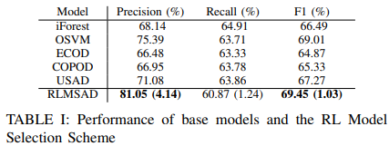
Accuracy (Precision) scores for the base models range from about 66% to 75%. All base models show a recall of about 63%. The F-1 scores of the base models range from about 65% to 69%.
Both the overall accuracy and F-1 scores are significantly improved in the proposed framework, with the RLMSAD accuracy and F-1 reaching 81.05% and 69.45%, respectively, demonstrating a significant improvement in anomaly detection performance.
2) Differences in a compensation setting
We investigate the effect of penalties on false positives (FP) and false negatives (FN) in the MDP formulation.
Effects of penalties for misidentification
We fixed the penalty for false negatives and varied the penalty for false positives. The results are shown in Table II. Increasing the penalty for false positives is to tell the model to be more cautious about its predictions. As a result, the model will report fewer false alarms and will only report anomalies when it is fairly confident in its prediction. In other words, the model is less sensitive to relatively small deviations in the sequence, which may improve accuracy. It also reports as anomalies only those data instances that differ significantly from the majority, thus covering less of the actual anomalies, which may result in a loss of reproducibility. This is evident in Table II, where recall scores decrease and accuracy scores increase as FP penalties increase.
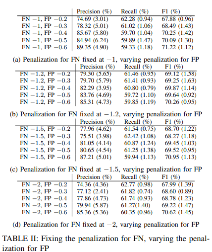
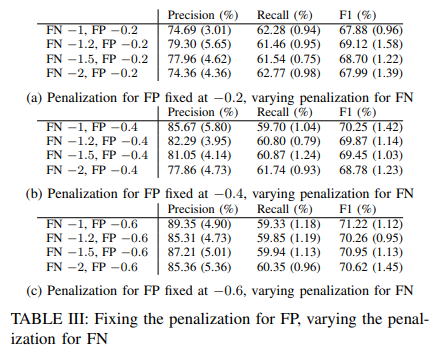
Effects of Penalties for False Negatives
We fixed the penalty for false positives and varied the penalty for false negatives. The results are shown in Table III. Increasing the penalty for false negatives encourages the model to be "bolder" concerning reporting anomalies. When the cost of false negatives (i.e., missing real anomalies) is high, the best strategy for the agent is to report as many anomalies as possible so as not to miss many real anomalies. In this case, the model is more likely to be hypersensitive to small deviations and lose accuracy. On the other hand, it is also more likely to cover more actual anomalies and achieve higher recall, since instances are more likely to be flagged as anomalies. This is demonstrated by the general decrease in accuracy scores and increase in recall scores in Table III.
3) Carve-out research
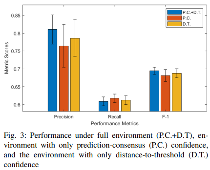
To investigate the effects of the two confidence levels, distance-threshold confidence (D.T.) and prediction-consensus confidence (P.C.), we performed a cut-and-dry approach. Here, two reinforcement learning environments were constructed in addition to the original reinforcement learning environment. In these two environments, each of the two confidence scores is removed from the state variables. We retrain the policy in each of these three environments and report the detection performance in Fig. 3. from Fig. 3, we can see that removing either of the two confidence scores results in a significant decrease in accuracy and F-1 score. only when the two confidence scores are considered as state components, the optimal performance is obtained when both of the two confidence scores are considered as state components.
summary
In this paper, we proposed a reinforcement learning-based model selection framework for time series anomaly detection.
Specifically, we first introduced two scores to characterize the detection performance of the base model: distance-threshold confidence and prediction-consensus confidence. Second, we formulated the model selection problem as a Markov decision process and used the two scores as state variables for RL. The goal was to learn a model selection policy for anomaly detection to optimize the long-term expected performance. Experiments on real-world time series demonstrated the effectiveness of the model selection framework of our method. In the future, we plan to focus on extracting appropriate data-specific features and embedding them into state transitions. This may enable RL agents to obtain more informative state descriptions and more robust performance.


Categories related to this article


