
WaveBound, A Regularization Method That Prevents Overlearning In Dynamic Time Series Data And Improves Prediction Accuracy
3 main points
✔️ This is a NeurIPS 2022 accepted paper. We address the problem of overlearning in time series prediction models. The regularization method WaveBound estimates appropriate error bounds for learning loss for each time step and feature at each iteration of the learning process.
✔️ WaveBound stabilizes the learning process and greatly improves generalization by making the model less focused on unpredictable data.
✔️ It outperforms SOTA on six real-world datasets.
WaveBound: Dynamic Error Bounds for Stable Time Series Forecasting
written by Youngin Cho, Daejin Kim, Dongmin Kim, Mohammad Azam Khan, Jaegul Choo
[Submitted on 25 Oct 2022 (v1), last revised 28 May 2023 (this version, v2)
Comments: Accepted by NeurIPS 2022
Subjects: Machine Learning (cs.LG)
code:
The images used in this article are from the paper, the introductory slides, or were created based on them.
summary
Recently, deep learning has shown remarkable success in time series prediction. However, due to the dynamics of time series data, deep learning still suffers from unstable learning and overlearning. This is because inconsistent patterns that appear in real-world data bias the model toward certain patterns, limiting generalization. To address the overlearning problem in time series forecasting, we propose a regularization method called WaveBound, which introduces a dynamic error bound on learning loss. This regularization method estimates appropriate error bounds on learning loss for each time step and feature at each iteration; WaveBound stabilizes the learning process and greatly improves generalization by allowing the model to focus less on unpredictable data. Extensive experiments show that WaveBound consistently improves existing models, including SOTA models, by a wide margin.
Introduction.
Time series forecasting has recently seen an increase in deep learning-based approaches, especially transducer-based methods, which have shown remarkable success. Nevertheless, inconsistent patterns and unpredictable behavior exist in real data, and forcing the model to fit patterns in such cases leads to unstable learning. In unpredictable cases, the model does not ignore them in learning, but rather suffers a significant penalty (i.e., learning loss). Ideally, a small learning loss should be applied to unpredictable patterns. This implies the need for proper regularization of the forecasting model in time series forecasting.
Recently, Ishida et al. argued that zero training loss introduces a high bias in training and hence overconfidence models and reduced generalization. To remedy this problem, they proposed a simple regularization called flooding, which explicitly prevents learning loss from decreasing below a small constant threshold called the flooding level. This study also focuses on the drawbacks of zero learning loss in time series forecasting. In time series forecasting, the model is forced to fit the unpredictable patterns that inevitably emerge, which almost always results in tremendous errors. However, the original flooding is not applicable to time series forecasting for two main reasons.
(i) Unlike image classification, time series prediction requires a vector output of prediction length × number of features. In this case, the original flooding considers the average learning loss without treating each time step and feature separately.
(ii) For time series data, error bounds should change dynamically for different patterns. Intuitively, higher errors should be allowed for unpredictable patterns.
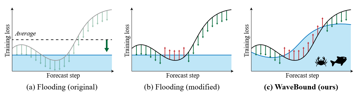
| Figure 1 Conceptual examples of different methods (a) The original flooding provides a lower bound on the average loss rather than considering each time step and feature separately. (b) Even though it provides a lower bound on training loss for each time step and each feature, a constant value lower bound cannot reflect the nature of time series forecasting. (c) The WaveBound method proposed by the authors provides a lower bound on training loss for each time step and feature. This lower bound is dynamically adjusted during the learning process to provide tighter error bounds. |
To properly address the overfitting problem in time series forecasting, the difficulty of the forecast, i.e., how unpredictable the current labels are, should be measured in the learning procedure. For this purpose, we introduce a target network updated with the exponential moving average of the original network, i.e., the source network. At each iteration, the target network can lead to a reasonable level of learning loss relative to the source network-the larger the error in the target network, the more unpredictable the pattern. In current research, slow-moving average target networks are commonly used to generate stable targets in a self-supervised setting. By using the learning loss of the target network as a lower bound, the authors derive a novel regularization method called WaveBound, which faithfully estimates error bounds for each time step and feature. By dynamically adjusting the error bounds, the proposed regularization prevents the model from overfitting certain patterns, further improving generalization. Figure 1 illustrates the conceptual differences between the original flooding and the WaveBound method. The originally proposed flooding determines the direction of all point update steps by comparing the average loss to its flooding level. In contrast, WaveBound uses dynamic error bounds on the learning loss to determine the direction of the update step for each point individually. The three main contributions of this study are:
- We propose a simple and effective regularization method, called WaveBound, that dynamically provides error bounds for learning loss in time series prediction.
- We show that the proposed regularization method consistently improves existing state-of-the-art time series forecasting models on six real-world benchmarks.
- Extensive experimentation will test the significance of adjusting error bounds by time step, feature, and pattern to address the problem of overfitting in time series forecasting.
introduction
time series forecast
Consider a rolling forecast setting with a fixed window size. The goal of time-series forecasting is to predict the past series xt = {zt-L+1, zt-L+2, ..., zt : zi∈RK } given a future series yt = {zt+1, zt+2, ..., zt : zi∈RK }, the task is to learn a forecaster g : RL×K → RM×K that predicts the future series yt = {zt+1, zt+2, ..., zt : zi∈RK } . We mainly deal with error bounds in multivariate regression problems where the input series x and the output series y originate from a basis density p(x, y). For a given loss function ℓ, the risk of g is R(g) := E(x,y)∼p(x,y) [ℓ(g(x), y)]. Since we do not have direct access to the distribution p, we instead use the training data 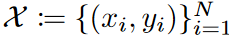 to minimize its empirical version
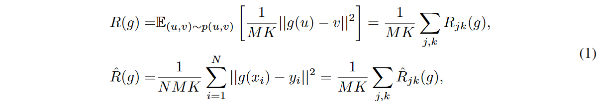
 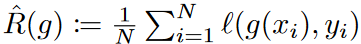 . In our analysis, we assume that the errors are independently homogeneously distributed. We use the widely used mean squared error (MSE) loss as the objective function. The risk can then be rewritten as the sum of the risks at each prediction step and feature:
WHEREAS, 
flooding
To address the problem of overlearning, Ishida et al. proposed flooding, which limits the learning loss above a certain constant. Given an empirical risk  and a manually explored lower bound b called the flood level, the authors instead minimize the flood empirical risk, defined as
![]()
The gradient update of the flooded empirical risk with respect to the model parameters is done in the same way as the gradient update of the empirical risk if  , and in the opposite direction otherwise. t ∈ {1, 2, . , T }, let
  be the empirical risk with respect to the t-th minibatch, then by Jensen's inequality

Thus, mini-batch optimization minimizes the upper bound on flooding empirical risk.
technique
Flooding in time series forecasts
We begin by explaining how the original flooding does not work effectively for the time series forecasting problem. We begin by rewriting equation (2) with the risk at each forecasting step and feature:

Flooding empirical risk constrains the lower bound on the average empirical risk of all forecast steps and characteristics by a constant value of b. However, for multivariate regression models, this regularization does not constrain each  independently. As a result, the effect of the regularization is concentrated on output variables that vary significantly in training.
For this situation, a modified version of flooding can be explored by considering the individual learning loss for each time step and feature. This can be done by subtracting the flood level b for each time step and each feature as follows

In this study, we refer to this flooding as constant flooding. Compared to the original flooding, which considers the average of the overall training loss, constant flooding separately constrains the lower bound of the training loss at each time step and feature by the value of b.
Nonetheless, it is not possible to account for the different predictive difficulties of each mini-batch. For constant flooding, it is difficult to properly minimize empirical risk variants in the batch-by-batch training process. As in Equation 3, the mini-batch optimization minimizes the upper bound of the flooded empirical risk. The problem is that for each t ∈ {1, 2, . , T }, each flooded risk term  differs significantly, the inequality becomes less tight. This happens frequently when the losses in each batch vary widely, since time series data usually contain a lot of unpredictable noise. To ensure the tightness of the inequality, the bounds of
  should be chosen adaptively for each batch.
WaveBound
As mentioned earlier, in order to adequately control empirical risk in time series forecasting, regularization methods should be considered under the following conditions
(i) Regularization should consider the empirical risk of each time step and each feature separately.
(ii) For different patterns, i.e., mini-batches, different error bounds should be explored in the training process for each batch.
To handle this, error bounds are obtained for each time step and each feature and adjusted dynamically at each iteration. Since it is impractical to manually search for different bounds for each time step and feature at each iteration, an exponential moving average (EMA) model is used to estimate error bounds for the different predictions.
Specifically, two networks are employed throughout the training phase: the source network gθ and the target network gτ, each with the same architecture but different weights θ and τ. The target network estimates an appropriate lower bound on the error relative to the source network's prediction, and its weights are updated with an exponential moving average of the source network's weights:
![]()
where α ∈ [0, 1] is the target attenuation rate. The source network, on the other hand, updates the weights θ using gradient descent updates in the direction of the gradient of the empirical risk  of the wave.
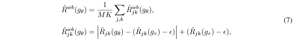
Here ε is a hyperparameter that indicates how far away the error bounds of the source network may be from those of the target network. Intuitively, the target network guides a lower bound on the learning loss for each time step and feature, preventing the source network from learning toward a loss lower than that lower bound. In other words, it overfits a pattern. Since the exponential moving average model is known to have the effect of ensembling the source network and remembering the training data visualized in previous iterations, the target network is able to resist instabilities caused mainly by noisy input data, while the error bounds of the source network are robustly estimated. Figure 2 illustrates the performance of the source and target networks in the WaveBound method.
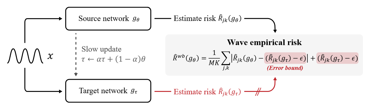
Figure 2 The WaveBound method provides dynamic error bounds on learning loss for each time step and feature using the target network. The target network gτ is updated with the EMA of the source network gθ. For the jth time step and kth feature, the learning loss is bounded by our estimated error bound  . That is, if the learning loss is below the error bounds, a gradient ascent is performed instead of a gradient descent. . That is, if the learning loss is below the error bounds, a gradient ascent is performed instead of a gradient descent. |
mini-batch optimization
For t ∈ {1, 2, . , T}, let  and
and  denote the empirical risk and empirical risk of the wave at the jth step and kth feature for the tth minibatch, respectively. Given a target network g*, by Jensen's inequality
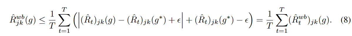
Thus, mini-batch optimization minimizes the upper bound on the empirical risk of waves.
Note that if g is close to g*, then the values of  are similar across mini-batches and a tight bound is placed on Jensen's inequality. We expect the EMA update to work so that this condition is satisfied, giving a tight upper bound on the empirical risk of waves in the mini-batch optimization.
MSE reduction
Given an appropriate ε, the MSE of the authors' proposed empirical risk estimator for the wave is smaller than the empirical risk estimator.
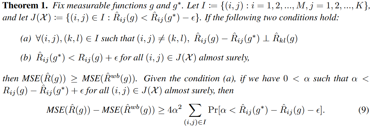
Intuitively, Theorem 1 states that the MSE of the empirical risk estimator can be reduced when the following conditions hold
(i) The network g* is sufficiently expressive and the loss difference between g and g* in each output variable is independent of the loss in the other output variables of g.
(ii) ˆ Rij(g∗) - ε is likely to lie between ˆ Rij(g) and Rij(g).
Since the learning loss of the EMA model is not easily below the test loss of the model, it is preferable to let g* be the EMA model for g. Then, ε can be chosen as a fixed small value so that the learning loss of the source model in each output variable is closely bounded below the test loss in that variable.
experiment
WaveBound with Predictive Model
For the multivariate setting, Autoformer, Pyraformer, Informer, LSTNet, and TCN were selected as baselines. In the univariate setting, we add N-BEATS [15] as baseline.
The dataset has six real-world benchmarks.
(1) The power transformer temperature (ETT) data set contains two years of data at 1-hour level (ETTh1, ETTh2) and 15-minute level (ETTm1, ETTm2) intervals collected from power transformers from two separate counties in China.
(2) Electricity (ECL) dataset consists of hourly electricity consumption for 321 clients over a two-year period.
(3) The Exchange dataset is a collection of features for eight countries on a daily basis.
(4) The Traffic dataset is hourly statistical data from various sensors in San Francisco Bay provided by the California Department of Transportation.
(5) The Weather dataset records four years (2010-2013) of data for 21 weather indicators collected at approximately 1,600 landmarks in the United States.
(6) The ILI dataset contains data on patients with influenza-like illnesses reported weekly by the Centers for Disease Control and Prevention from 2002 to 2021, describing the ratio of patients seen for ILI to the total number of patients.
・Multivariate Results
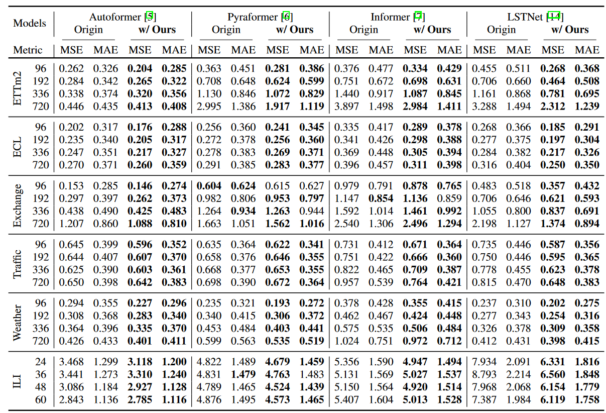
Table 1 shows the performance of the methods in terms of mean squared error (MSE) and mean absolute error (MAE) in a multivariate setting. It can be seen that the authors' methods show consistent improvement over a variety of forecasting models, including the most recent methods. In particular, WaveBound improves both MAE and MSE for the ETTm2 dataset by 22.13% (0.262 → 0.204) for MSE and 12.57% (0.326 → 0.285) for MAE for M = 96. In particular, LSTNet improves performance by 41.10% (0.455 → 0.268) for MSE and 27.98% (0.511 → 0.368) for MAE. In the long-term ETTm2 prediction setting (M = 720), WaveBound improves Autoformer performance by 7.39% (0.446 → 0.413) for MSE and 6.20% (0.435 → 0.408) for MAE. In all experiments, the authors' method consistently shows performance gains for a variety of prediction models.
| Table 1: WaveBound results in the multivariate setting. All results are averages of three trials. |
・Single-variable results
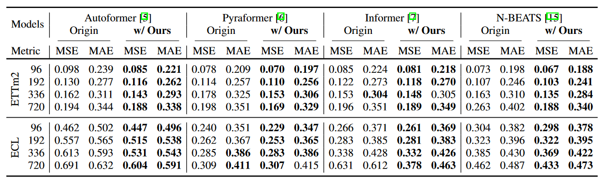
As reported in Table 2, WaveBound also shows excellent results in the univariate setting. In particular, in N-BEATS, specifically designed for univariate time series forecasting, the authors' method improves the performance of the ETTm2 dataset by 8.22% (0.073 → 0.067) in MSE and 5.05% (0.198 → 0.188) in MAE when M = 96. For the ECL dataset, the Informer with WaveBound shows an improvement of 40.10% (0.631 → 0.378) for MSE and 24.35% (0.612 → 0.463) for MAE when M = 720.
| Table 2: WaveBound results in the univariate setting. All results are averages of three trials. |
・generalization gap
To identify overfitting, one can examine the generalization gap, which is the difference between training loss and test loss. To verify that the authors' regularization is indeed preventing overfitting, Figure 3 shows both training and test losses for models with and without WaveBound. without WaveBound, test losses begin to increase rapidly, indicating a high generalization generalization gap. In contrast, with WaveBound, we observe that test loss continues to decrease, indicating that WaveBound successfully addresses overfitting in time series forecasting.
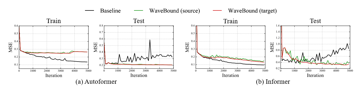
| Figure 3 Learning curves for models with and without WaveBound on ETTm2; without WaveBound, the learning loss for both models decreases while the test loss increases (see black line). In contrast, test loss for the model with WaveBound continues to decrease after learning more epochs. |
Significance of dynamically adjusting error bounds
In WaveBound, error bounds are dynamically adjusted for each time step and each feature at each iteration. To test the importance of these dynamics, WaveBound is compared to the original flooding and to constant flooding, which uses a constant value for the flooding level.
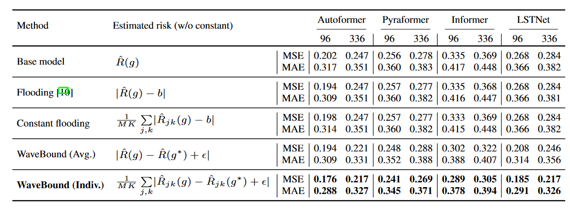
Table 3 compares the performance of flooding regularization with various proxy values for empirical risk. The original flooding bounds the empirical risk by a constant, while the constant flooding bounds the risk for each feature and time step independently. The flooding level b of the regularization method is set to {0.00, 0.02, 0.04, . .0.40} space, searched for a fixed value of b. As expected, no improvement was achieved using fixed constant values. The model trained with separately bounded errors for each output variable significantly outperformed the other baselines, specifically demonstrating the effectiveness of the authors' proposed WaveBound method. The test errors of the different methods at each time step are shown in Figure 4. At all time steps, WaveBound shows improved generalization compared to the original flooding and constant flooding, which underscores the importance of adjusting error bounds in time series forecasting.
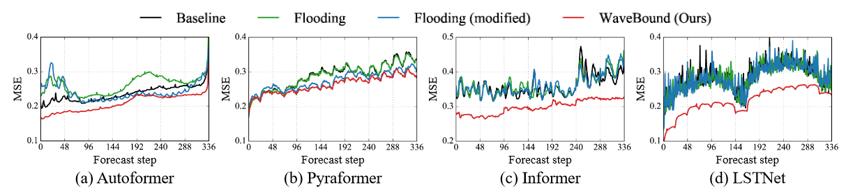
| Figure 4 Testing errors for models trained with different regularization methods on the ECL dataset. Compared to the original flooding and constant flooding, the test errors for WaveBound are consistently lower at all time steps, indicating that the authors' method is successful in improving generalization regardless of the range of predictions. |
| Table 3 Results for variations of flooding regularization on the ECL dataset. Prediction accuracy when training the source network with different surrogates is compared to empirical risk. All results are averages of three trials, with constant values b of {0.00, 0.02, 0.04, . .0.40}, which is faithfully explored within {0.00, 0.02, 0.04, ..., 0.40}. |
Flatness of loss landscape
Visualization of the loss landscape is introduced to assess how well the model generalizes. The flatter the loss landscape of a model, the more robust and generalizable it is known to be. Figure 5 illustrates the loss landscape for Autoformer and Informer. Visualizing the loss landscape using filter normalization and evaluating the MSE of each model for a fair comparison, we can observe that the model with WaveBound exhibits a smoother loss landscape compared to the original model. In other words, WaveBound flattens the loss landscape of the time series prediction model and stabilizes the learning.
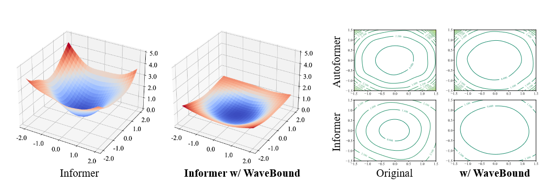
| Figure 5 Autoformer and Informer loss landscapes with and without WaveBound applied to the ETTh1 dataset; WaveBound flattens the loss landscape of both models and improves the generalizability of the models. |
Related Research
time series forecast
Various approaches have been proposed for the time series forecasting task, based on different principles. Statistical approaches can provide theoretical guarantees as well as interpretability. Autoregressive integral moving averages and prophets are the most representative of statistical approaches. Another important class of time series forecasting is the state-space models (SSMs), which incorporate structural assumptions into their models and learn about the potential dynamics of the time series data. However, due to its superior results in long-range forecasting, deep learning-based approaches are largely considered the leading solution for time series forecasting. Recurrent neural networks (RNNs) and convolutional neural networks (CNNs) have been introduced into time series forecasting to model the time dependence of time series data. Temporal convolutional networks (TCNs) are also being considered to model temporal causality. a combined SSM and neural network approach has also been proposed. deepSSM uses RNNs to estimate state space parameters. Linear latent dynamics are efficiently modeled using Kalman filters, and methodologies for modeling nonlinear state variables have also been proposed. Other recent approaches include SSM using Rao Blackwellized particle filters and SSM using duration switching mechanisms.
Recently, transformer-based models have been introduced for time series forecasting because of their ability to capture long-range dependence. However, applying the self-attention mechanism increases the complexity of the sequence length L from O(L) to O(L2). Several attempts have been made to reduce this computational burden, including LogTrans, Reformer, and Informer, which redesign the self-attention mechanism into a sparse version and reduce the complexity of the transformer Haixu et al. have developed a new version of the self-attention mechanism called Autoformer, called proposed a decomposition architecture with an autocorrelation mechanism to provide serial connections. To model different ranges of time dependence, pyramidal attention modules are proposed in Pyraformer. However, these models still fail to generalize due to learning strategies that force the model to fit all inconsistent patterns that appear in real data. The main focus of this study is to provide appropriate error bounds to prevent models from over-fitting certain patterns during the learning process.
regularization technique
Overlearning is one of the critical concerns of overparameterized deep learning networks. It can be identified by the generalization gap (the gap between learning loss and test loss). Several regularization techniques have been proposed to prevent overlearning and improve generalization. Weight parameter decay, early stopping, and dropout are commonly applied to avoid high biases in deep learning networks. In addition to these techniques, regularization methods specifically designed for time series prediction have also been proposed. Recently, Flooding, which explicitly prevents zero learning loss, has been introduced; Flooding improves the generalizability of a model by providing a lower bound on the learning loss, called the Flooding level, which allows the model to not perfectly fit the training data. This study also attempts to address zero learning loss in time series forecasting. However, we found that average loss in time series forecasting does not work as well as expected. Time series forecasting requires careful selection of appropriate error bounds for each feature and time step. Also, constant Flooding levels may not be suitable for time series forecasting, where the difficulty of forecasting changes with each iteration of the mini-batch learning process. To address these issues, the authors proposed a new regularization that fully accounts for the nature of time series forecasting.
summary
The authors proposed a simple and effective regularization scheme for time series forecasting called WaveBound, which uses a relaxed moving average model to provide dynamic error bounds for each time step and feature. Extensive experiments with real-world benchmarks showed that the authors' regularization scheme consistently improves existing models, including state-of-the-art models, and addresses overlearning in time series prediction. We also validated the generalization gap and loss landscape to discuss the effect of WaveBound in learning overparameterized networks. We believe that the significant performance improvement of the authors' method indicates that regularization should be designed specifically for time series prediction.


Categories related to this article