Easy! High Accuracy! Attractiveness Of The Anomaly Detection Model PatchCore

Object Detection 12/07/2023

3 main points
✔️ Achieve SOTA on the MVTec dataset, an anomaly detection problem benchmark!
✔️No need to train the CNN for the feature extraction part by utilizing pre-trained models
✔️ Efficient sampling of features obtained from the CNN allows for faster inference

Towards Total Recall in Industrial Anomaly Detection
written by Karsten Roth, Latha Pemula, Joaquin Zepeda, Bernhard Schölkopf, Thomas Brox, Peter Gehler
(Submitted on 15 Jun 2021 (v1), last revised 5 May 2022 (this version, v2))
Comments: Accepted to CVPR 2022
Subjects: Computer Vision and Pattern Recognition (cs.CV)

code：

The images used in this article are from the paper, the introductory slides, or were created based on them.

Introduction.

The anomaly detection problem is the task of detecting data with different behavior among a large number of data. This paper deals specifically with the anomaly detection problem for industrial image data.

In the real world, it is relatively easy to acquire normal images, while it is difficult to acquire abnormal images with various possible patterns. Therefore, various models have been proposed to identify abnormal images by learning only normal images.

In this paper, we propose a model called PatchCore, which achieves SOTA on the benchmark MVTec dataset_[1]. The most important feature of PatchCore is that it leverages features from pre-trained models and does not require any additional training for image feature extraction.

The following is a detailed description of PatchCore.

PatchCore

Overall Model

First, an overview of PatchCore is provided.

PatchCore calculates the degree of abnormality based on the distance between the feature vectors of the normal image contained in the Memory Bank and the feature vectors of the image (test data) to be judged, and determines whether the image is normal or abnormal. It can also obtain the anomaly degree for each pixel of the image, allowing it to detect anomalous areas.

Next, we briefly describe the learning and inference flow in PatchCore.

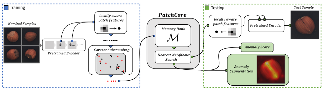
The left side of the above figure (blue dotted box) shows the learning process and the right side (green dotted box) shows the inference process.

Only normal images are used in training. The image is passed through the trained CNN model to obtain a feature vector for each patch (①), then sampling is performed and the selected feature vectors are stored in the Memory Bank (②).

Inference is performed using the Memory Bank in which feature vectors of normal images are accumulated in this way. During inference, the image is also passed through the trained CNN model to obtain a feature vector for each patch (①). Then, based on the distance between the obtained feature vectors and the feature vectors in the Memory Bank, the degree of abnormality is calculated for each image and pixel (③).

Now that we have seen the big picture of PatchCore's learning and inference, we will provide a detailed explanation below. In particular, we will explain the three parts circled in the explanation above.

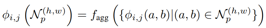
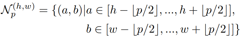
Locally aware patch features

The first is Locally aware patch features, which obtains a feature vector for each patch from the image.

PatchCore acquires feature vectors from images using a CNN model _[2] that has already been trained on a dataset called ImageNet. This part of the CNN model is not trained again on the dataset for which we want to determine normality or abnormality.

Adaptive average pooling is then performed on the feature vectors obtained from the learned CNN model. The process up to this point can be expressed in the following equation.

The question is which feature vector from which layer of the learned CNN model should be used. One possible candidate is the final layer.

The final layer provides the most aggregated, high-abstraction (high-level) feature vectors and has been used in several prior studies. However, this paper points out two problems with using feature vectors obtained from the final layer.

Loss of local features
- While the feature vectors in the deeper layers are at a higher level, the resolution is lower due to repeated convolution and pooling. This means that local (fine-grained) features may be lost.
Being a feature biased towards different domains (ImageNet classification problems)
- The learned model has been trained on a task that is different in domain from the inference target, and the deeper layers are likely to contain more features that are specific to that task. Therefore, we argue that it is not appropriate to use a final layer feature vector that is heavily influenced by tasks with different domains.

Therefore, in this paper, we propose to obtain feature vectors from the middle layer of the learned model in order to obtain feature vectors at the highest possible level and with the least influence of prior learning, and verify the effectiveness of this method through experiments.

The graph below shows the relationship between the layers of the learned model from which feature vectors are obtained (horizontal axis: the smaller the number, the shallower; the larger the number, the deeper) and the accuracy in the anomaly detection task (vertical axis: the larger (higher) the accuracy).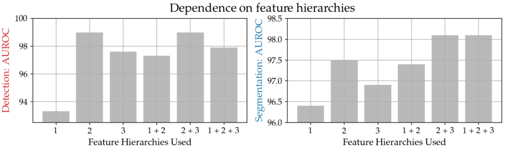

The above graph shows that the accuracy is indeed high for patterns that include "2," the middle layer. This result indicates that PatchCore acquires feature vectors from the "2" and "3" layers (2+3)_[3].

Coreset-reduced patch-feature memory bank

The second is the Coreset-reduced patch-feature memory bank, which stores the feature vectors obtained in (1) in the Memory Bank.

As the number of training data increases, more data must be stored in the Memory Bank, increasing the inference time required to evaluate test data and increasing the amount of memory needed to store the data.

Therefore, this paper proposes to use Coreset Sampling to perform sampling on the feature vectors obtained in (1) and store them in the Memory Bank.

The sampling method is represented by the following equation, where M is the set of feature vectors before sampling and _MC is the set of feature vectors after sampling.

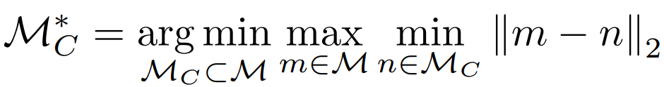
The above equation means that sampling should be performed so that the maximum minimum distance is the smallest in the feature vector (m) before sampling and the feature vector after sampling.

However, this optimization problem is NP-hard and requires a lot of computation time to obtain the optimal solution. Therefore, in this paper, the following two innovations are used to obtain a near-optimal solution more quickly.

Approximation by the greedy method
- The methods used in previous studies are employed.
Dimensionality reduction by random projection
- Reducing the dimensionality of feature vectors reduces the computational complexity of the optimization problem described above, and the Johnson-Lindenstrauss complement is a good basis for accurate dimensionality reduction.

This paper examines the effectiveness of Coreset Sampling.

The following figure applies Coreset Sampling to dummy data and visualizes the results.

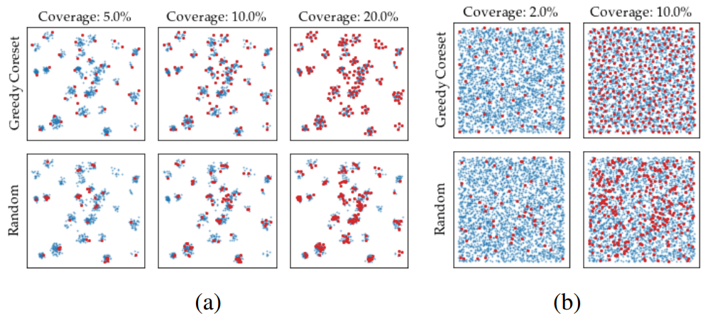
The following chart compares the dimensionality reduction performed on the two dummy data sets (a) and (b) using Random and Coreset Sampling, where Coverage represents the percentage reduction from the original sample data. It can be seen that Coreset Sampling above is more efficient than Random Sampling below.

The following graph also shows the relationship between the reduction ratio (horizontal axis) and accuracy (vertical axis) in the anomaly detection task for each dimension compression method.

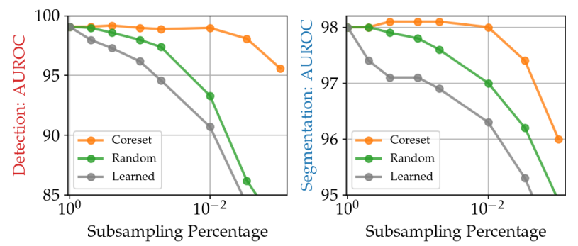
The above graph shows that in the case of Random, the accuracy drops significantly when the reduction rate ^{reaches about 10-2}, but in the case of Coreset (Sampling), the accuracy does not drop that much. Therefore, Coreset Sampling is an efficient sampling method that can reduce the number of data while retaining the features necessary for anomaly detection.

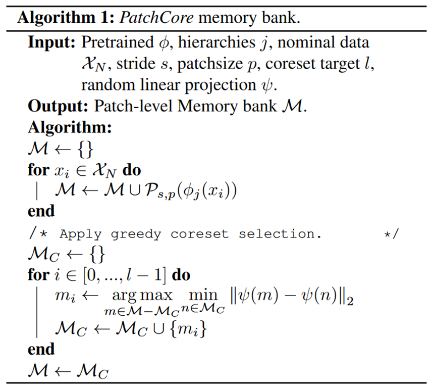
Finally, the entire algorithm for storing in the Memory Bank that we have described is shown below.

(3) Anomaly Detection with PatchCore

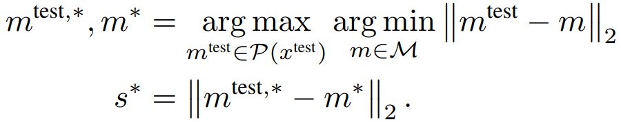
The third is Anomaly Detection with PatchCore, which uses the memory bank obtained in (2) to calculate the degree of anomaly in the image (test data) to be discriminated.

First, as in training, test data images are passed through the trained CNN model to obtain a feature vector for each patch.

Anomaly (s*) is calculated from the feature vector (mtest ⁾ for each patch of test data and the feature vector (m) stored in the Memory Bank according to the following formula.

experiment

experimental setup

In this paper, we test the effectiveness of the proposed method on three different datasets.

The first is the MVTec dataset. It is widely used as a benchmark and has 15 categories, including Bottle, Cable, and Grid. This dataset is the main focus of this study.

The second is the Magnetic Tile Defects (MTD) dataset. The task is to detect cracks and scratches in porcelain tile images.

The third is the Mini Shanghai Tech Campus (mSTC) dataset _[4], which consists of pedestrian videos of 12 different scenes and is tasked with detecting anomalous behaviors such as fighting and bicycling.

valuation index

The AUROC (Area under the Receiver Operator Curve) is used as a measure of performance in distinguishing normal from abnormal images. PRO is less sensitive to the size of the abnormal area.

result

We will begin with the results of the MVTec dataset _[5].

The table below shows the results of the comparison with conventional methods in AUROC.

Additionally, the table below shows the pixelwise AUROC results.

The results for PatchCore are shown when the memory bank subsampling is varied by 25%, 10%, and 1%, respectively, indicating that PatchCore is more accurate for both AUROC and pixelwise AUROC. We can also see that decreasing the percentage of memory bank subsampling does not cause much of a drop in accuracy.

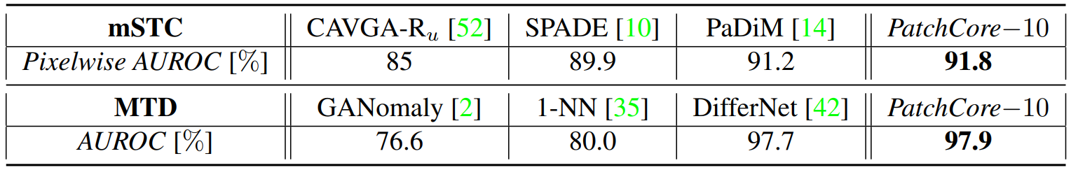
Results for mSTC and MTD are shown in the table below. The results on these data sets also exceed the accuracy of conventional methods.

inference time

The following table shows the accuracy (AUROC, pixelwise AUROC, PRO) and inference time for each method on the MVTec dataset.

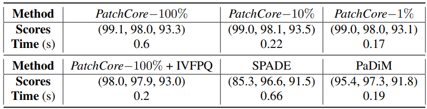
If we look at the results of PatchCore, we can see that the inference time varies greatly depending on the percentage of Coreset Sampling. In particular, the results with 1% sampling are not much different from those with 100% sampling, indicating that faster inference is possible while maintaining a higher accuracy than with conventional methods.

summary

We introduced PatchCore, which achieved SOTA on the MVTec dataset.

I found it very attractive that the pre-trained model eliminates the need to train the feature extraction part (CNN) and that Coreset Sampling can reduce the inference time by efficiently sampling features.

In addition, although this paper focused on the problem of anomaly detection in industrial image data, it can be applied to a variety of fields.

supplement

[1] SOTA is achieved in (image)AUROC, which is the accuracy of distinguishing normality and abnormality in an image.
[2]Among the pre-trained models by ImageNet, ResNet50 and WideResnet-50 are used in this paper.
[3] When two layers are used, the number of dimensions (resolution) of the feature vectors obtained is different. Therefore, bilinear interpolation is applied to the low-resolution feature vectors to align the number of dimensions.
[4] The video frames of the original STC dataset are subsampled every 5 frames.
[5] The results for the average of 15 categories are shown.