The Latest Comprehensive Review Of Activation Functions!

Survey 28/06/2022

3 main points
✔️ There are five types of activation functions (sigmoidal, ReLU, ELU, learning, and other), each with its challenges.
✔️ There is no such thing as the "best activation function", and there is an optimal activation function for each data and model.
✔️ ReLU is an excellent place to start, but Swish, Mish, and PAU are also worth a try.

A Comprehensive Survey and Performance Analysis of Activation Functions in Deep Learning
written by Shiv Ram Dubey, Satish Kumar Singh, Bidyut Baran Chaudhuri
(Submitted on 29 Sep 2021 (v1), last revised 15 Feb 2022 (this version, v2))
Comments: Submitted to Springer.
Subjects: Machine Learning (cs.LG); Neural and Evolutionary Computing (cs.NE)

code：

The images used in this article are from the paper, the introductory slides, or were created based on them.

first of all

The purpose of a neural network (NN) is to transform nonlinearly separable input data into more linearly separable features by learning. The activation function should have the following features

Bringing in nonlinearities to help optimize the network.
Do not excessively increase computational costs.
Does not inhibit gradient flow.
Maintain data distribution.

Evolution of the activation function

The linear function $ y = cx $ is a simple activation function (called an identity function when $c$ is constant and $c=1$).

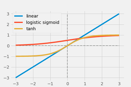
The red graph above is the linear function, along with the logistic sigmoid function (blue) and the hyperbolic tangent (green). The important point is that linear functions cannot introduce nonlinearity into the network.

Logistic sigmoid hyperbolic tangent series

$$\text { Logistic Sigmoid }(x)=\frac{1}{1+e^{-x}}$$

$$ \operatorname{Tanh}(x)=\frac{e^{x}-e^{-x}}{e^{x}+e^{-x}} $$

The above two functions are early popular non-linear activation functions, inspired by neurons in the biological sense (note: biological neurons obey the all-or-nothing rule, so they only output 0 or 1, and nothing in between). Logistic Sigmoid limits the output to $[0,1]$, but the output does not change much concerning the size of the input (saturated output), which causes gradient vanishing. Also, the fact that the output is not zero-centric makes it unsuitable for optimization.

In contrast, $ \operatorname{Tanh}(x) $ is zero-centered and has output $[-1,1]$; however, the gradient vanishing problem remains unsolved The gradient vanishing problem is still not solved.

ReLU Series

The Rectified Linear Unit (ReLU) has become the state of the art (highest quality, highest performance, SOTA) activation function due to its simplicity and improved performance.

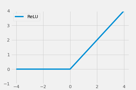
$$ \operatorname{ReLU}(x)=\max (0, x)= \begin{cases}x, & \text { if } x \geq 0 \\ 0, & \text { otherwise }\end{cases} $$

However, ReLU had a problem of under-utilization of negative value input.

Exponential Unit Series

Logistic Sigmoid and Tanh's problem was saturated output, where the output is narrow ($[0,1]$) relative to the input range from infinitesimal to infinity, and ReLU does not make good use of negative inputs. This is where the Exponential Linear Unit (ELU) comes in.

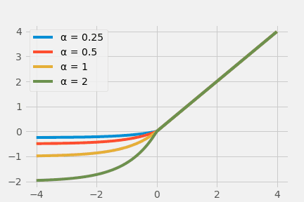
$$ \operatorname{ELU}(x)= \begin{cases}x, & x>0 \alpha \times\left(e^{x}-1\right), & x \leq 0\end{cases} $$

Learning and adaptation system

The activation functions of Sigmoid, Tanh, ReLU, and ELU systems mentioned so far were designed by hand, so to speak, and may not extract the complexity of the data sufficiently.

$$ \operatorname{APL}(x)=\max (0, x)+\sum_{s=1}^{S} a_{i}^{s} \max \left(0,-x+b_{i}^{s}\right) $$

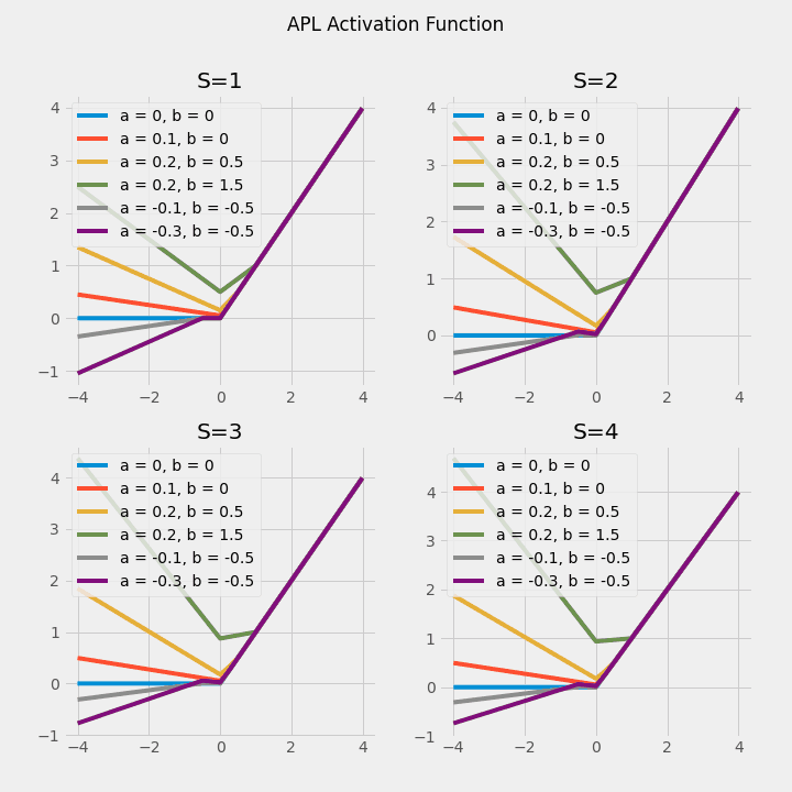
In APL $ a_i $ and $ b_i $ are the learning parameters, and the activation function itself changes (note: the graphs for S=3 and S=4 look the same, but upon closer inspection they are different).

the others

Many other activation functions have now been proposed, including Softplus functions, stochastic functions, polynomial functions, kernel functions, etc.

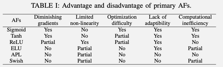
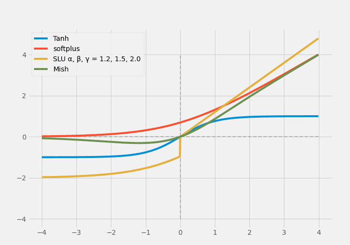
The advantages and disadvantages are summarized in the table above, from left to right: gradient vanishing, nonlinearity, difficulty of optimization, lack of adaptability, and computational cost The table is shown in the left column.

Logistic Sigmoid/Tanh based activation function

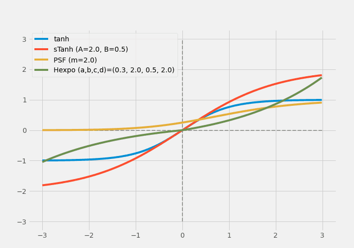
A scaled hyperbolic tangent (sTanh) is proposed for the narrow output range and gradient vanishing problem of $ \operatorname{Tanh}(x) $.

$$ \operatorname{sTanh}(x)=A \times \operatorname{Tanh}(B \times x) $$

The parametric sigmoid function is proposed as a differentiable and continuous bounded function.

$$ \operatorname{PSF}(x) = (\frac{1}{1+\exp(-x)})^m $$

Similarly, shifted log-sigmoid and rectified hyperbolic secant were proposed, but the saturated output and gradient disappearance problems remained. scaled sigmoid and penalized Tanh were proposed, but gradient vanishing was still unavoidable.

Later, a method called noisy activation function, in which the activation function is given a random number to improve the gradient flow was proposed to deal well with the saturated output problem. The Hexpo function solved most of the gradient vanishing problems.

$$ \operatorname{Hexpo}(x)= \begin{cases}-a \times\left(e^{-x / b}-1\right), & x \geq 0 \\ c \times\left(e^{x / d}-1\right), & x<0\end{cases} $$

The sigmoid-weighted linear unit (SiLU) and improved logistic sigmoid (ISigmoid) were proposed at the same time to solve the saturated output and gradient vanishing problems The linearly scaled hyperbolic tangent (LiSHT), Elliott, and Soft-Root-Sign (SRS) were also proposed at the same time.

Many activation functions in the Sigmoid/Tanh system have tried to overcome the gradient vanishing problem, but in many cases, the problem has not been completely solved.

Rectified Activation Functions

The rectified linear unit (ReLU) is a simple function that outputs a constant function concerning positive inputs and zero concerning negative inputs (output is also zero when input is zero).

$$ \operatorname{ReLU}(x)= \begin{cases}x, & \text { if } x \geq 0 \\ 0, & \text { otherwise }\end{cases} $$

So the derivative can only be 1 (positive input) or 0 (negative input), so Leaky ReLU (LReLU) is modified to return a small value instead of 0 for negative inputs Leaky ReLU (LReLU) is modified to return a small value for negative inputs instead of zero.

$$\operatorname{LReLU}(x)= \begin{cases}x, & x \geq 0 \times x, & x<0\end{cases}$$

The problem with LReLU, however, is that it does not know whether 0.01 is the correct coefficient, and Parametric ReLU (PReLU) avoids this by learning the coefficients.

$$ \operatorname{PReLU}(x)= \begin{cases}x, & x \geq 0 \times x, & x<0\end{cases} $$

However, PReLU had a drawback that it was prone to overlearning.

$$ \operatorname{RReLU}(x)= \begin{cases}x, & x \geq 0 \\ R \times x, & x<0\end{cases} $$

Randomized ReLU (RReLU) is a method to randomly select coefficients.

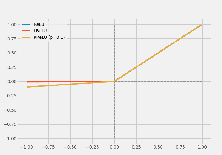
(Note: The coefficients are so small that they almost overlap)

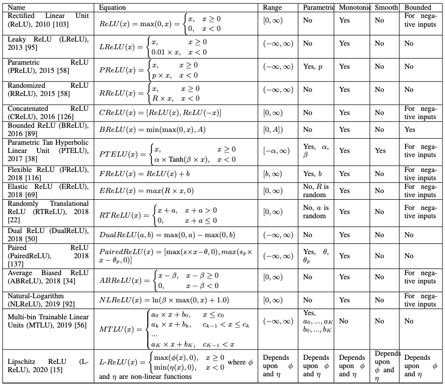
Various other variants of ReLU have been proposed.

Exponential Activation Functions

The activation function of the Exponential system tackles the gradient vanishing problem in ReLU.

$$\operatorname{ELU(}x)= \begin{cases}x, & \text { if } x>0 \alpha \times\left(e^{x}-1\right), & \text { otherwise }\end{cases}$$

The ELU is saturated for large, differentiable, negative inputs, which makes it more robust to noise than the Leaky ReLU or Parametric ReLU.

$$ \operatorname{SELU}(x)=\lambda \times \begin{cases}x, & x>0 \\ \alpha \times\left(e^{x}-1\right), & x \leq 0\end{cases} $$

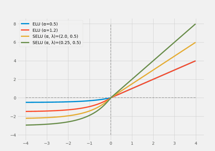
(Note: in regions where x > 0, the blue and red colors overlap.)

Scaled ELU (SELU) uses a hyperparameter for scaling so that it does not saturate for huge positive inputs.

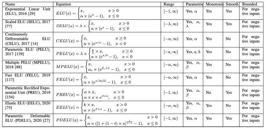
The variants of ELUs have been summarized above, all of which are considered to deal with saturation for large values and computational cost.

Learning/Adaptive Activation Functions

Many of the aforementioned activations were not adaptive.

$$\operatorname{APL}(x)=\max (0, x)+\sum_{s=1}^{S} a_{s} \times \max \left(0, b_{s}-x\right)$$

Adaptive Piecewise Linear (ALP) is a hinge-shaped activation function, where a and b are learnable parameters and S is a hyperparameter representing the number of hinges. S is a hyperparameter representing the number of hinges, meaning that each neuron has a different value of a and b, and each neuron has its activation function The activation function of a and b is the hyperparameter that represents the number of hinges.

Swish was proposed by Ramachandran et al. and found by automatic search.

$$ \operatorname{Swish}(x)=x \times \sigma(\beta \times x) $$

$\sigma$ is a sigmoidal function; Swish is made to look like ReLU.

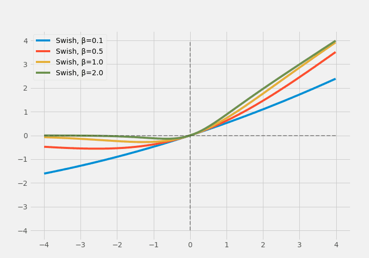
Later Swish was extended to ESwish.

$$ \operatorname{ESwish}(x)=\beta \times x \times \sigma(x) $$

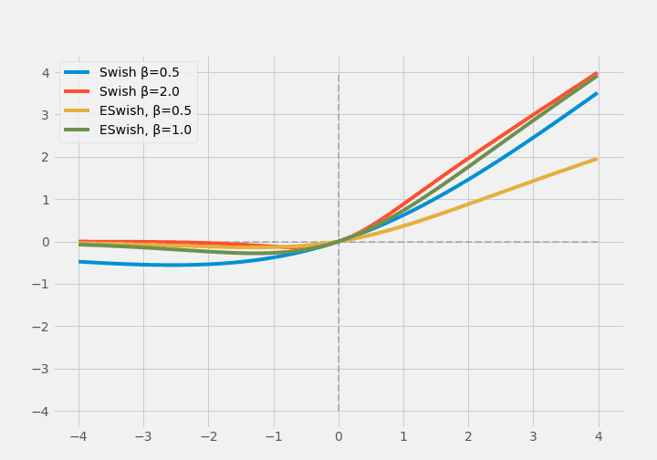
(Note: $\beta=1.0$ matches Swish and ESwish, so I'm breaking apart the $\beta$ values for each. But they still look very similar)

Learning and adaptive activation functions are defined by having an underlying activation function and adding learnable variables to it. For example, the adaptive activation function using Parametric ReLU and Parametric ELU described above has $\sigma(w \times x) \times \operatorname{PReLU(x)} + (1-\sigma(w \times x)) \times $ There is one defined as $\operatorname{PELU}(x)$ ($\sigma$ is an S-shaped function where $w$ is a learnable variable).

Alternatively, each neuron may use a different activation function. This does not mean that each neuron uses a different activation function as a result of different values of the learnable variables, but different activation functions. In some studies, each neuron chooses between ReLU and Tanh and learns the choice itself.

Nonparametrically learning AFs, which are activation functions that do not use hyperparameters that can be learned, are reported to be not activation functions that can be written in a single equation as described above, but activation functions that themselves are very shallow neural networks. This is called hyperactivations, and the network is called a hyper network.

Learning and adaptive activation functions are a recent trend. They are being studied to deal with more complex and nonlinear data, but of course, the computational cost is increasing. The following table summarizes the learning and adaptive activation functions.

Other activation functions

A. Softplus activation function

Softplus function was proposed in 2001 and was often used in statistics.

$$ \operatorname{softplus}(x)=\log{(e^x+1)}$$

Subsequently, the popularity of deep learning led to the common use of softmax functions, which are attractive because they can output probability values for each class in a classification task.

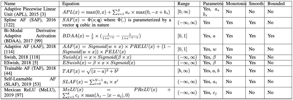
Since Softplus is smooth and differentiable, the Softplus Linear Unit (SLU) is a ReLU-like version of it.

$$ \operatorname{SLU}(x)=\begin{cases} \alpha \times x, & x>0 \\ \beta \times \log{(e^x+1)} - \gamma, & x \leq 0\end{cases} $$

$\alpha,\beta,\gamma$ are trainable parameters.

The activation function called Mish is a non-monotonic activation function, again using Softplus, and Mish also uses Tanh.

$$ \operatorname{Tanh}(x)=\frac{e^{x}-e^{-x}}{e^{x}+e^{-x}} $$

$$\operatorname{Mish}(x)=x \times \operatorname{Tanh(\operatorname{Softplus(x)})}$$

Mish is smooth and non-monotonic. Recently, it is used in YOLOv4. However, it has a drawback that it is computationally complex and thus computationally expensive.

B. Stochastic activation function

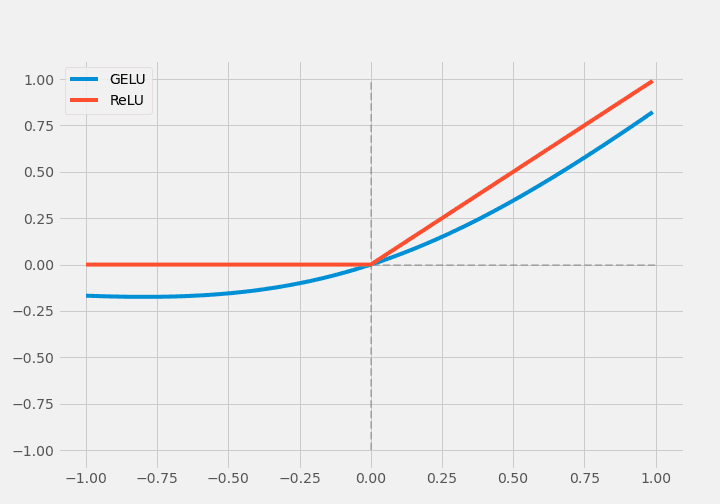
RReLU, EReLU, RTReLU, and GELU are the few activation functions in this category. GELU (Gaussian Error Linear Unit) takes into account the nonlinearity by stochastic regularization.

$$\operatorname{GELU}(x)=x P(X \leq x)=x \Phi(x)$$

Φ is defined as $\Phi(x) \times I x+(1-\Phi(x)) \times 0 x=x \Phi(x)$, which is called stochastic regularization. In the original work, it is approximated as $0.5 x\left(1+\tanh \left[\sqrt{2 / \pi}\left(x+0.044715 x^{3}\right)\right]\right)$.

C. Multinomial activation function

The Smooth Adaptive Activation Function (SAAF) was developed as a piecewise polynomial activation function, which combines two symmetric power functions on the linear part of ReLU, improving the performance of ReLU.

$$ \operatorname{SAFF}(x)=\sum_{j=0}^{c-1} v_{j} \mathrm{p}^{j}(x)+\sum_{k=1}^{n} w_{k} \mathrm{~b}_{k}^{c}(x) $$

where

$$ \begin{aligned} \mathrm{p}^{j}(x) &=\frac{x^{j}}{j !} , \quad \mathrm{b}_{k}^{0}(x)=\mathbb{1}\left(a_{k} \leq x<a_{k+1}\right) \mathrm{b}_{k}^{c}(x) &=\underbrace{\iint \ldots \int_{0}^{x}}_{c \text { times }} \mathrm{b}_{k}^{0}(\alpha) \mathrm{d}^{c} \alpha \end{aligned}$$

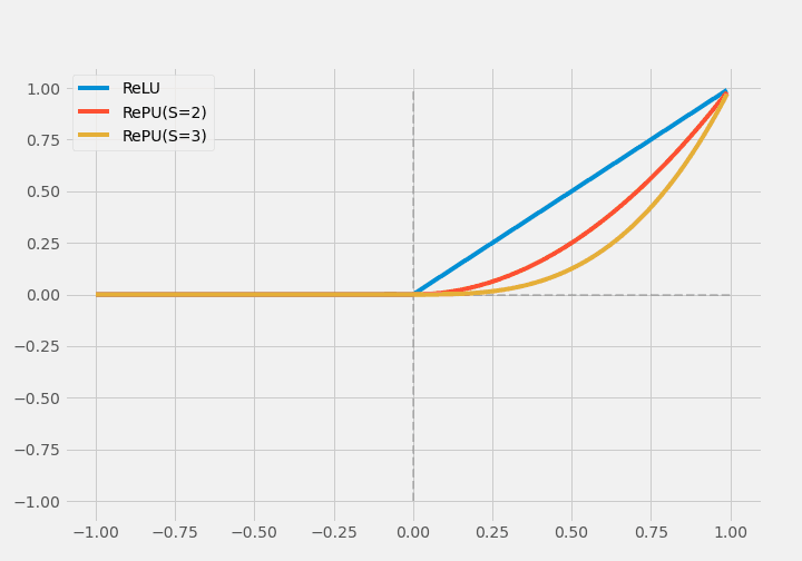
ReLU is also extended to a Rectified Power Unit (RePU) with $y=X^S$ in the $ x>0 $ part ($S$ is a hyperparameter). However, the susceptibility to gradient vanishing, unboundedness, and asymmetry are also drawbacks of RePU.

Recently, the Padé Activation Unit (PAU) has been developed using the Padé approximation method.

$$ \operatorname{PAU}(x) = P(x) / Q(x) $$

PAU is defined above, where $P(x)$ and $Q(x)$ are $m$- and $n$-degree polynomials, respectively, and are hand-designed.

$$F(x)=\frac{P(x)}{Q(x)}=\frac{\sum_{j=0}^{m} a_{j} x^{j}}{1+\sum_{k=1}^{n} b_{k} x^{k}}=\frac{a_{0}+a_{1} x+a_{2} x^{2}+\cdots+a_{m} x^{m}}{1+b_{1} x+b_{2} x^{2}+\cdots+b_{n} x^{n}}$$

In the original book, it is defined as above.

Performance comparison of each activation function

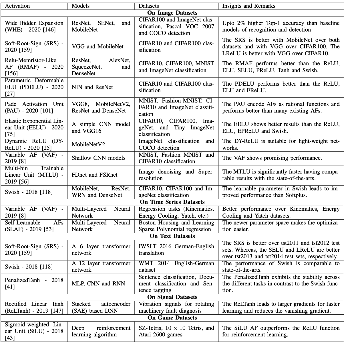
The table above lists the activation functions that have already been reported to achieve SOTA. Among the ones described so far are the Padé Activation Unit (MNIST in VGG8) and Swish (CIFAR10 and CIFAR100 in MobileNet and ResNet). The datasets vary from images, time series, text, etc., but except for Swish, there are no identical activation functions that achieve SOTA when the datasets are changed.

Experiments on CNN

We implemented the models and compared them, not in the paper. The dataset is CIFAR10.

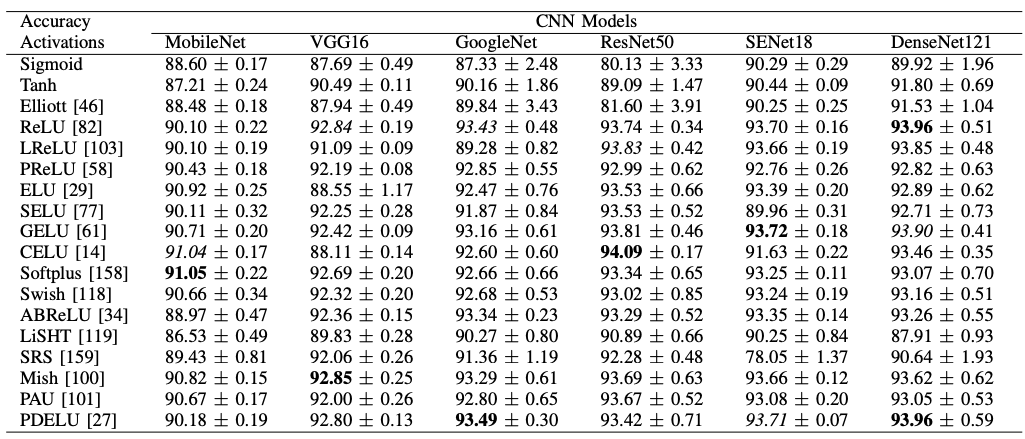
Although the dataset is the same, we can see that as the model changes, so does the appropriate activation function.

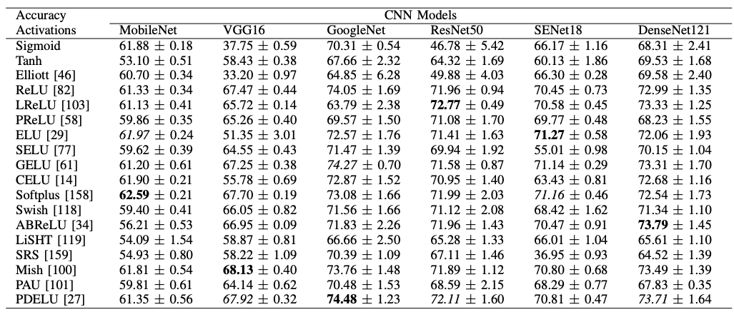
The above results are obtained by changing the dataset to CIFAR100; the best performing activation functions for MobileNet, VGG16, and GoogleNet are the same as for CIFAR10, but the results for ResNet50, SENet18, and DenseNet121 have changed (although the best performing activation functions for The best performing activation function in CIFAR10 is the same as in CIFAR10, the results have changed in ResNet50, SENet18, and DenseNet121.)

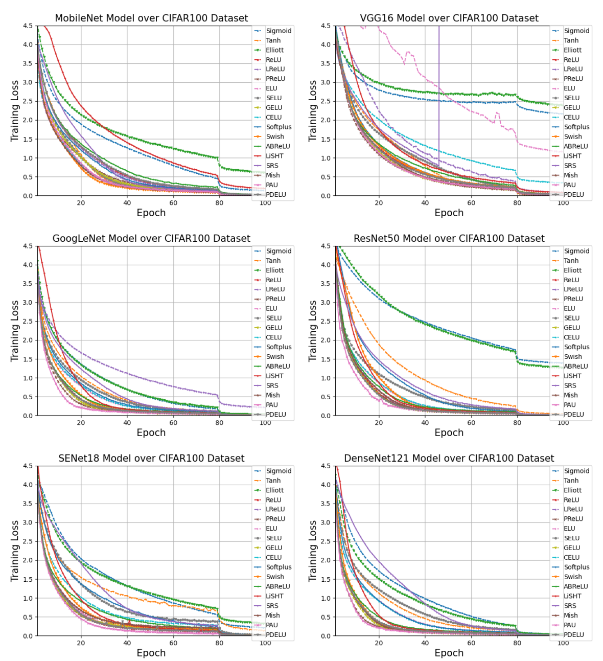
This graph shows the loss for each model. The activation functions are distinguished by color. In the graph legend, it seems that if the activation function is less than or equal to ReLU, we can get the loss close to zero over time. So let's compare the time taken for 100 epochs.

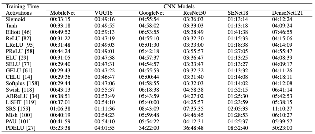
Only PDELU is taking longer than the rest of the pack.

$$\operatorname{PDELU}(x)= \begin{cases}x, & x>0 \\ \alpha \times\left([1+(1-t) \times x]^{\frac{1}{1-t}}-1\right), & x \leq 0\end{cases}$$

(Note: For PDELU, the original work is not open access and the meaning of the variable $t$ is unconfirmed. My apologies.)

Conclusion.

In this paper, we have conducted an extensive survey and experiments on activation functions. Different types of activation functions have been reported and in this paper, we have specifically discussed their performance in deep learning. The conclusions of this paper are summarized as follows.

Advances have been made in the activation functions of logistic-sigmoidal hyperbolic tangent series for nonzero mean and gradient vanishing. However, the advances have increased the computational cost.
ReLU series have made progress against underutilization of negative inputs, bounded nonlinearity, and unbounded output. However, in most cases, ReLU is better, and ReLU (or Leaky ReLU, Parametric ReLU) is still the first choice of researchers.
The focus of the Exponential series is to take advantage of negative inputs. The only problem is that most of them are not smooth.
Learning and adaptive sequences are a recent trend, but the problem is, not surprisingly, the setting of the underlying function and the number of parameters.

And here are the authors' recommendations

If you want to reduce the learning time, you can use an activation function where the average of the outputs is zero and utilize positive and negative inputs.
The key is to choose a model that is commensurate with the complexity of the data. The activation function is just a bridge between the complexity of the data and the expressive power of the model, and if the gap between the two is too large, it will fail (over-adaptation or under-learning).
Logistic sigmoid hyperbolic tangent series should not be used for CNNs. This kind of activation function is valid for RNNs.
ReLU is a good choice. But Swish, Mish, and PAU should also be tried.
ReLU, Mish, and PDELU should be used for VGG16 and GoogleNet.
ReLU, LReLU, ELU, GELU, CELU, and PDELU should be used for image classification tasks for models with residual connections.
In general, parametric activation functions can be fitted to the data faster. PAU, PReLU, and PDELU are especially recommended.
PDELU, SRS increases the learning time.
The accuracy of ReLU, SELU, GELU, and Softplus decreases when the training time is short. I can assure you that.
Exponential series are more likely to take advantage of negative inputs.
Tanh, SELU is good for natural language processing; PReLU, LiSHT, SRS, and PAU are also good.
PReLU, GELU, Swish, Mish, and PAU are considered good for speech recognition.