MegazordNet: Stock Prediction With Statistics And Machine Learning
3 main points
✔️ Statistics x Machine Learning to improve the accuracy of stock predictions!
✔️ Higher accuracy than traditional statistical and ML-based algorithms
✔️ Expand the possibilities of stock prediction
MegazordNet: combining statistical and machine learning standpoints for time series forecasting
written by Ilya Tolstikhin, Neil Houlsby, Alexander Kolesnikov, Lucas Beyer, Xiaohua Zhai, Thomas Unterthiner, Jessica Yung, Andreas Steiner, Daniel Keysers, Jakob Uszkoreit, Mario Lucic, Alexey Dosovitskiy
(Submitted on 23 Jun 2021)
Comments: Published on arxiv.
Subjects: Statistical Finance (q-fin.ST); Artificial Intelligence (cs.AI); Computational Engineering, Finance, and Science (cs.CE); Machine Learning (cs.LG)
code:
The images used in this article are either from the paper or created based on it.
first of all
Forecasting financial time series is considered to be a challenging task due to its chaotic nature. Recent literature has shown that the combined use of statistics and machine learning may improve the accuracy of forecasting compared to single solution methods. With these considerations in mind, we propose MegazordNet, a framework for exploring statistical features in financial series in combination with structured deep learning models for time series forecasting.
related research
Despite the longstanding dominance of statistical modeling, ML is now vastly applied to FTSF (Financial Time Series Forecasting).
Parmezan et al. (2019) evaluate different statistical and ML algorithms for TSF using 40 synthetic and 55 real datasets. According to the results obtained for various metrics, results show that the statistical approaches could not outperform the ML-based techniques with statistical differences.
One of the authors' contributions was to organize a repository containing all the datasets used in their analysis to facilitate the replication of their work and its evaluation against other modeling techniques.
Makridakis et al. (2018b) presented the results of an M4 competition that aimed to study new ways to improve the accuracy of TSFs and how such learning can be applied to advance the theory and practice of forecasting. The competition presented statistical, ML, and "hybrid" approaches to modeling complex TS data from different disciplines.
The results reinforce the idea that no single method is suitable for all problems, but that a combination of several methods can usually provide good results.
In their study, Hu et al. (2018) evaluated different optimization methods to determine the optimal set of parameters for an artificial neural network created to model the trends of the US stock market. They used data from the S&P 500 index and the DJIA index as well as data from Google Trends to model the TS.
The results showed that for financial forecasting, there is an impact of exploring different external sources based on public and investor sentiment, such as Google Trends, as well as the value of TS.
Bai et al. (2018) compared simple CNN results with RNNs to see which architecture performs better.
They found that their results showed that CNNs could also be used as a benchmark for these types of problems.
Lin et al. (2017) proposed a pipeline in which CNN extracts salient features from local raw data of TS while LSTM models existing long-range dependencies in historical data trends.
They propose a joint representation that can predict the trend of TS using a feature fusion layer.
Most of the existing solutions focus only on specific areas of predictive research, such as ML and statistical modeling. Since this strategy may not be optimal for tackling complex tasks such as TSFs, we hypothesize that combining statistical methods with the learning capabilities of DLs can improve predictive performance in FTSFs.
proposed method
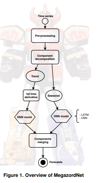
We present our proposal, called MegazordNet, for the TSF.
In this case, we want to predict the next day's closing price, so we will use only this variable to model TS and treat this as a univariate problem.
Preprocessing and decomposition of time series components
After the training partition is obtained, the input data is to remove the missing entries from the TS. It is subjected to a preprocessing step. The input is then decomposed into trend and seasonal components.
Since financial TSs represent complex data patterns and are often influenced by external factors, decomposing the original series into different components should result in a data representation that is easier to model with forecasting algorithms.
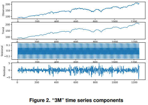
The simple moving average method is used to extract the trend, seasonality, and residual components.
For this purpose, we adopt a window size of 10 days. An example of the applied operation is shown in Figure 2. After decomposition, the trend and seasonal components are modeled separately to learn the best model for each of them and to obtain individual forecasts. Furthermore, to account for the non-stationarity of financial markets, we apply first-order differentiation to the trend component. We ensure that the trend model can only learn the variation from one-time observation to the other. In the final trend forecast, MegazordNet will add the results of the learned trend variability model to the previous trend observation.
We chose not to model the residual component (Residual) because there are many small chaotic fluctuations in financial stocks that may disturb the final results of the proposed approach. For the forecasting of the Trend and Seasonal components, an additive model can be applied to obtain the forecast of the next time step as the sum of the forecasts of the separate components.
component prediction
To explore the state-of-the-art of TSFs, we employ CNNs and LSTMs in this study. Since these models are familiar to the readers, we omit them here.
Data and experimental setup
In this section, we describe the resources and methodology used to address the TSF task.
data
The S&P 500 dataset shows the economic transactions of the S&P 500 Index over a five-year period. The index covers the 503 most economically prominent companies in the United States, with approximately 1258 daily observations recorded for each company. In total, 606,800 samples make up this data set. Removing the incomplete samples from it, the total number comes to 601,011. Table 1 shows the features included in this data set.

Experiment setup
With the aim of evaluating the performance of different approaches to TSFs, we adopt Hold-out and 8:2 as suggested in recent literature.
Comparison between the proposed method and the conventional method
Table 2 summarizes the algorithms compared against MegazordNet in this study, along with their settings; for both MegazordNet and the compared methods, the hyperparameter settings are fixed regardless of the TS considered. The results empirically show that satisfactory results are obtained in most cases. In the table, the tuples following the ARIMA variants are of the form (p, d, q), where p is the order of the regression model (number of time lags), q is the degree of differentiation, and q is the order of the moving average model. Furthermore, α is the decay coefficient of the SES, w is the window of time intervals considered in the MA and k-NN-TSP, and k is the number of neighbors employed in the k-NN-TSP.

Evaluated variants of MegazordNet
As mentioned earlier, in this preliminary study, we consider two types of neural networks for TSF: LSTMs and CNNs. Since MegazordNet builds different predictors for both trend and seasonal components, four different combinations of these neural networks are possible.
The acronyms of the MegazordNet variants are listed in Table 3 along with their meanings.

valuation index
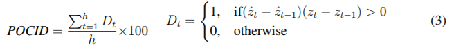
For the performance measures, these are the Mean Squared Error (MSE), Theil's U (TU) coefficient, and the Hit Rate Prediction of Change in Direction (POCID). We omit the mean squared error (MSE) and Theil's U (TU) coefficient. (Please check the original publication)
The Hit Rate Prediction of Change in Direction (POCID) calculates the number of times a method correctly predicts the direction of change in a stock index, that is, whether it will rise or fall. For this calculation, we used the POCID indicator shown in Equation 3.
Results and Discussion
The discussion focuses on statistical tests to account for the fact that the range of shares in each company is different, i.e., the value varies widely. Furthermore, the difficulty of forecasting varies across series. Therefore, we omit details when summarizing the performance measures for all 148 series covered in this study. We do, however, present a case study of APH, a stock that showed some odd behavior in its TU coefficient during our analysis.
Statistical comparison of each algorithm
The results obtained for the MSE are described in this section. This analysis is illustrated in Figure 5. The algorithms with the highest accuracy have the lowest ranking. Algorithms for which there is no statistical difference in the resulting MSE (α=0.05) are connected by horizontal bars; the MegazordNet variant occupies the first position.
The first group consisted of CNN-based variants, while LSTM-based variants made up the second group. Regardless of the algorithm that constitutes the trend, the seasonal component does not seem to have a significant impact on the ranking of MegazordNet variants.
In all cases, the model using only the trend predictor did not differ from the model using the seasonal predictor. However, in such applications, accuracy to the nearest cent is important. Therefore, the use of MegazordNetC,C is recommended when the primary concern is to reduce the MSE.

Among the traditional algorithms for time series forecasting, the autoregressive model and SES are in the third most accurate group of algorithms.
RW generated the smallest MSE despite the lack of statistical improvement; given the randomness of RW's method and its ranking, we believe that none of the statistical-based algorithms adequately captured the movement of the stock being evaluated.
The TU coefficient compares each algorithm to a trivial baseline prediction that uses the previous day's observation as the baseline; the smaller the TU, the higher the performance improvement obtained by the considered algorithm. Figure 6 shows the results of the statistical tests on TU. Again, the same ranking is observed between the different models of MegazordNet.
The CNN-based model achieved the best value of TU, while the LSTM-based model again reached the second-best position. All MegazordNet variants that use the same type of neural network for the trend component are grouped together.

However, the ranking changed for the traditional TS prediction algorithm. RW had the best accuracy in the MSE but is the lowest in this analysis. This result is expected because we apply a random deviation from the last observed timestep. In general, the autoregressive model tended to reproduce the last day's observations with some deviation. For this analysis, SES is the best traditional approach, followed by k-NN-TSP and MA.
To illustrate, we compare the average TU values obtained by the MegazordNet variants for each TS with the minimum TU values obtained by the other solutions. Even without taking the best model, MegazordNet is able to outperform the best of the traditional prediction algorithms in the majority of cases.
Considering the POCID, the Megazord variant again reached the highest position in the ranking as shown in Figure 7. It can be said that this was the best method for predicting the upward and downward trends of the stocks considered in this study. There were some changes in the order of MegazordNet. However, the differences in the order were small and not statistically significant.

We also compared the average POCID performance of the proposed method with that of the best method, as shown in Figure 9. When POCID is considered, MegazordNet shows the best performance regardless of the TS under consideration. The average POCID achieved by MegazordNet is, in most cases, 50% the which is higher than that of the random guessing strategy. Thus, it ranks above random guessing strategies and is on average better than some other models.

Case Study: APH Stock
The characteristics of TS are shown in Figure 10a: the stock price dropped sharply around September 2014. A magnified view of this phenomenon is shown in Figure 10b. It is difficult for any learning algorithm to model such a situation. As a result, the first derivative component shown in Figure 10c illustrates this fact: MegazordNet uses this representation to learn the unit interval variability of TS.
When we looked for the phenomena that occurred in APH on other platforms such as Yahoo Finance, we found that the observed declines appeared to be inconsistent with the data set employed. Therefore, given the practical application of the methodology, a more robust data extraction procedure needs to be adopted. In addition, MegazordNet was biased towards erroneous behaviors because the online learning mechanism was not employed in this experiment.
Due to the non-stationary features observed, online learning of MegazordNet should be considered in the future.

summary
In this work, a new framework called MegazordNet was proposed for FTSF, which combines statistical analysis and ANNs.MegazordNet, despite the simplicity of its basic design with respect to the data transformation procedures employed, and regardless of the performance metrics considered, is able to It statistically outperforms traditional statistical and ML-based algorithms. However, the accuracy is still about 60% on average, which is very difficult for financial time series forecasting.


Categories related to this article
.JPG)


