TSDFNet For Time Series Forecasting With An Attentive Feature Value Fusion Mechanism
3 main points
✔️ In time series forecasting, a lot of effort was required to set features of interest by domain knowledge to improve accuracy.
✔️ TSDFNet uses an autoregression mechanism and an attentive feature fusion mechanism to extract important features without any feature engineering.
✔️ We validated it on more than a dozen datasets and confirmed its outstandingly superior prediction performance compared to conventional methods such as Seq2Seq, LSTM-SAE, etc.
Temporal Spatial Decomposition and Fusion Network for Time Series Forecasting
written by Liwang Zhou, Jing Gao
(Submitted on 6 Oct 2022)
Comments: Published on arxiv.
Subjects: Machine Learning (cs.LG); Artificial Intelligence (cs.AI)
code:
The images used in this article are from the paper, the introductory slides, or were created based on them.
summary
To achieve better results in time series forecasting, feature engineering is necessary, and decomposition is an important one. Standard time series decomposition, however, lacks flexibility and robustness, and a single decomposition approach often cannot be used for many forecasting tasks. Traditional feature selection relies heavily on existing domain knowledge, lacks a generic methodology, and requires a lot of effort. However, many time series prediction models based on deep learning generally suffer from interpretability issues, and "black box" results do not inspire confidence. Addressing the above issues is the motivation for this paper. In this paper, we propose TSDFNet as a neural network with an autoregression mechanism and an attentive feature fusion mechanism. It abandons feature engineering as a preprocessing convention and creatively integrates it as an internal module with deep learning models. The autoregression mechanism gives TSDFNet an extensible and adaptive decomposition capability for any time series, allowing users to choose their basic functions to decompose into time series and generalized spatial dimensions. The attentive feature fusion mechanism can capture the importance of external variables and their causal relationship to the target variable. It can also automatically suppress unimportant features and reinforce valid features, so users do not have to struggle with feature selection. In addition, TSDFNet makes it easy to look into the "black box" of deep neural networks through feature visualization and analyze prediction results. Demonstrating improved performance over existing widely accepted models on over a dozen datasets, three experiments demonstrate the interpretability of TSDFNet.
Introduction.
Time series forecasting plays an important role in many areas such as economics, finance, transportation, and weather, empowering people to foresee opportunities and guiding decision-making. Therefore, it is important to increase the versatility of time series models and reduce the complexity of modeling while maintaining performance. In the field of time series forecasting, multivariate and multistage forecasts form one of the most difficult challenges. Currently, there is no universal method to address the problem of multivariate and multistage time series forecasting. Therefore, data analysts need to have specialized background knowledge (domain knowledge).
Feature engineering is typically used to preprocess data before modeling. In the field of feature engineering, time series decomposition is the classical method of decomposing a complex time series into a large number of predictable sub-series, such as STL for seasonal and trend decomposition, EEMD for ensemble empirical mode decomposition, and EWT for the empirical wavelet transform. In addition, feature selection is another important step. Complex tasks usually require several auxiliary variables to aid in the prediction of the target variable. Rational selection of additional features is critical to model performance, as the introduction of redundant additional features can degrade model performance.
This is because the introduction of redundant additional features can degrade the performance of the model. In addition, how to select the appropriate decomposition method and important additional features is a difficult problem for the data analyst.
On the other hand, despite the large number of models proposed, each has its shortcomings. The majority of deep learning-based models are difficult to understand and provide unconvincing predictive results. However, models like ARIMA and xgboost, which have a sound mathematical foundation and offer interpretability, cannot compete with deep learning-based models in terms of performance.
Therefore, it is necessary to break with conventional practices and devise new methods to handle these problems. In this study, we have developed a new neural network model called TSDFNet, based on an autolysis mechanism and an attentive feature fusion mechanism. Decomposition and feature selection are integrated as internal modules of the deep model to reduce complexity and increase adaptability. Higher-order statistical features of the data may be captured by the model's robust feature representation capabilities, making it applicable to data sets in a variety of domains.
In summary, the contributions are as follows
- Temporal Decomposition Network (TDN) is a scalable and adaptive network that decomposes time series on the time axis and allows users to customize basis functions for specific tasks.
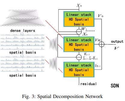
- The Spatial Decomposition Network (SDN) uses high-dimensional external features as decomposition basis functions to model the relationship between external and target variables.
- We also proposed the Attentive Feature Fusion Network (AFFN), which has an automatic feature selection function and can capture the importance and causality of features. This saves users the trouble of feature selection and allows arbitrary basis functions to be used in the autoregressive network without worrying about the degradation of model performance due to the introduction of invalid features.
- TSDFNet has yielded interpretable results for a multifaceted data set and has significantly improved performance compared to many previous models.
Related Research
The field of time series forecasting has a long history and many excellent models have been developed. Some of the best-known traditional methods include ARIMA and exponential smoothing; the ARIMA model turns a non-stationary process into a stationary process by differencing and can be further extended to a VAR to address multivariate time series forecasting problems, and its interpretability and ease of use are the main reasons for its popularity. Another effective forecasting technique is exponential smoothing. This smoothes univariate time series by giving the data exponentially decreasing weights over time.
Since time series forecasting is essentially a regression problem, various regression models can also be used. There are also machine learning-based methods such as decision trees and support vector regression (SVR).
In addition, ensemble methods, which employ multiple learning algorithms to achieve better prediction performance than can be achieved with only one of the constituent learning algorithms, are also effective tools for sequence prediction. Examples of such methods include random forests and adaptive lifting algorithms (Adaboost).
Deep learning has become popular in recent years, and neural networks have achieved success in many fields. It uses back-propagation algorithms to optimize network parameters.LSTM (Long Short-Term Memory) and its derivatives show great power with sequential data, overcoming the shortcomings of RNN (Recurrent Neural Network) Deep autoregressive networks (DeepAR) use stacked LSTMs to perform iterative multistage prediction, and Deep state-space models (DSSM) use a similar approach to perform predefined muti-stage prediction. Seq2Seq (Sequence to Sequence) typically uses a pair of LSTMs or GRUs as encoders and decoders. The encoder maps the input data into a fixed-length semantic vector in hidden space, and the decoder reads the context vector and attempts to predict the target variable in a stepwise fashion. Temporal convolutional networks (TCNs) can also be effectively applied to the sequence prediction problem and can be used as an alternative to the popular RNN family of methods, being faster and having fewer parameters compared to RNN-based models.
It is faster and has fewer parameters than RNN-based models using causal convolution and residual connections. Attention mechanisms appear as an encoder-decoder-based improvement and can be easily extended to self-attention mechanisms as the core of further Transformer models.
technique
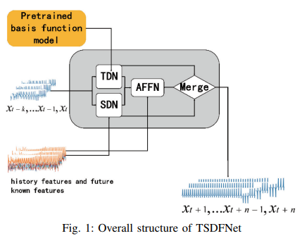
The architecture of this network is shown in Fig. 1. It consists of two main parts: the first is an autoregressive network including TDN and SDN. The feature fusion network (AFFN) is an additional component.
A. Autolysis network
The structure of the autoregression network includes two decomposition modules: one is the temporal decomposition network TDN, which employs custom basis functions to decompose sequences in the temporal dimension. The other is a spatial decomposition network SDN, which uses exogenous features as basis functions to decompose sequences in a generalized spatial dimension. The main goal is to decompose complex sequences into simple and predictable sequences.
TDN can capture signal features using multiple basis functions pre-trained with different parameters, such as triangular basis, polynomial basis, and wavelet basis.
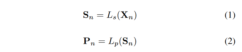
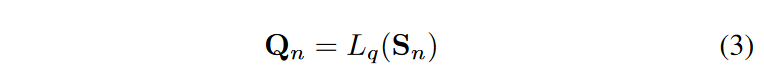
The architecture of TDN is shown in Fig. 2. n recursive decomposition units exist in TDN. The (n+1)th unit accepts as input each input Xn and outputs two intermediate components Wn and Vn. Each decomposition unit consists of two parts: a stacked fully connected network Ls maps the data to the hidden space and generates a semantic vector Sn, and the basis expansion coefficients are predicted forward and backward through two sets of fully connected networks Lp and Lq, respectively. The process is as follows.
The procedure is as follows
The other is a set of pre-trained basis function models. This is a function of the time vector t = [-w, -w + 1, h -1, h]/L functions. where L = w + h + 1, w is the time history window length of the drive sequence and h is the time window length of the target sequence. This time vector is fed to different pre-trained models, Cn = [sin(-kt), cos(-kt),. , cos(kt), sin(kt)], trigonometric functions with different frequencies defined by Cn = [t, t2, t3. .tk], polynomial functions with different degrees defined by Cn = [-w/L. .0] and Cpn when t = [0. .h/L] and Cpn for t = [0...h/L], which are used to fit past and future data, respectively. Their coefficient matrices Pn and Qn determine the importance of each basis function.
- The final output of the nth block is defined as

- The input to the next block is defined as follows

- The original signal X0 = [xt-w, xt-w+1..., xt-1] continues to remove the backward feature component Wn, and ideally the residual is random noise that no longer has feature information.

- The forward output of each decomposition unit is integrated as follows, resulting in a TDN output.

- The hyperparameters N of the model are defined as the number of decomposition layers and depend on the type of basis functions chosen and are repeatable for each basis function. The weights of these basis function networks can be adjusted once more for different tasks to adapt to diverse scenarios.

- Fig. 3 shows the Spatial Decomposition Network (SDN). Its structure is similar to that of the TDN. The difference is that SDN employs external features mapped to higher dimensions as basis vectors CpnandCqn. Details are as follows.

- Here, Ep is the past additional features and Eq is the future additional features; Ln is a stacked fully connected module that maps past and future additional features to higher dimensions, respectively. It employs embedding to transform some discrete features and 0 to fill in missing features. In addition, it is important to note that the autoregression module provides flexibility for dealing with univariate time series. The Spatial Decomposition Network (SDN) module can be disabled, or the SDN can be enabled to accept feature components from other methods such as EMD as input.
B. Attentive feature fusion network
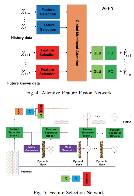
As shown in Fig. 4, the feature selection module is designed to perform instance-by-instance variable selection, groups of decision units repeatedly suppress irrelevant features, and the multi-head attention block accepts the results of the feature selection module as input and further models global relationships The outputs are then used to model the global relationship between the features and the features. Finally, outputs are obtained at each time step by the GLU and FC, where the GLU attempts to suppress invalid portions of the input data.
As shown in Fig. 5, we designed a feature selection block that includes a mask generator and a feature separator.
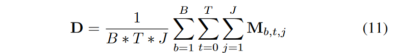
A learnable mask generator is employed to generate a dynamic mask M with explainability indicating the importance of each dimensional feature. The mask at decision step j takes as input the features separated at step j - 1. Mj = entmax(h(aj-1), where h is a learnable function and entmax can map a vector to a sparse probability, similar to a conventional softmax. A series of basis function features can be filtered by M, where Mj=0 means that the feature input at this step is irrelevant to the prediction task as this sample, and the filtered features M - X is fed to the next decision step. In general, we are interested in which features contribute more to the target variable. If the batch size of the dataset is B, the time length is T, and the decision step is J, the importance distribution is given by
The feature separator has a shared layer, consisting of GLU, and LN; layer normalization (LN) is a technique to normalize the distribution of the middle layer. The output of the shared layer s of the feature separator is divided into two parts [s1, s2], one of which, f1(s1), is used as input to the mask generator and the other, f2(s2), as the output of the j-th level decision, where f1 is the FC layer and f2 is Relu, if s2 < 0, it contributes If s2 < 0, it has no contribution to the current decision output.
Multiple Attention, as it is well known, is as follows
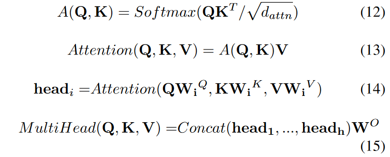
Among these, MultiHead(Q, K, V) represents the attention function; Softmax is the probability distribution function, with parameters dattn to normalize the features on a scale; K is the key for a given time segment; V is the value of the feature; Q is the input query feature; WO is the network output weight is the weight of the network output. The model uses a self-attention mechanism to learn the correlations between each feature at various times. For a given target element query, the weight coefficients of each key for the target are obtained by calculating the similarity between queries Q and K, then performing a weighted sum of the targets to obtain the final attention value. By dividing the model into several heads, and forming different subspaces, we can focus on different aspects of the features. In this model, Q is the high-dimensional feature of all historical information output from the feature selection module, while K and V are the high-dimensional features of future known information.
experiment
To evaluate the proposed TSDFNet, we chose typical models such as TCN based on causal convolution, Lstnet based on CNN and RNN, Seq2Seq based on attention and LSTM, and Lstm-SAE based on stacked autoencoders and thorough Comparisons were made.
A. Implementation
The experiment is conducted on an Ubuntu system using the Pytorch framework. Hardware configuration is Intel(R) Core(TM) I7-6800K CPU @ 3.40 GHZ, 64 GB memory, GeForce GTX 1080 GPU.
First, multiple synthetic basis functions with different parameters k are constructed to give diversity to the model yi = Ci(kt), including trigonometric and polynomial functions. These models are 3-layer fully connected networks trained with L2 loss. Each dataset has 10000 training samples, the training period is set to 100, and the batch size in the experiment is set to 40.
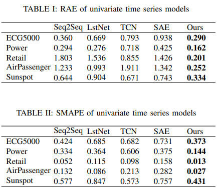
The second step is to train the TSDFNet using the ADAM optimizer with an initial learning rate of 0.0001. The dropout rate is set to 0.1 for better generalization and the batch size is set to 32. To avoid overfitting, early stopping is employed and the learning process is terminated if there is no loss degradation within 10 epochs. The evaluation metrics are RAE and SMAPE.
B. Univariate Time Series Forecasts and Result Analysis
Univariate results for five representative data sets are listed in Table I and Table II. Because ECG and energy consumption are quasi-periodic, it is difficult to predict peaks and valleys of uncertainty. Retail sales and airline passenger volume data are difficult to reliably predict cycles and trends because of the small training sample. Sunspot eruptions, on the other hand, are periodic but cannot be predicted because of their extremely long time horizon.
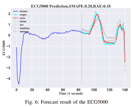
ECG5000
The data set consists of 5000 electrocardiograms (ECGs) from the UCR time series data, 4500 samples for training, and 500 samples for testing. Each sample in the sequence is 140-time points. In this experiment, the first 84 time steps are used as input and the last 56 time steps are predicted as the outcome. The results are shown in Fig. 6.
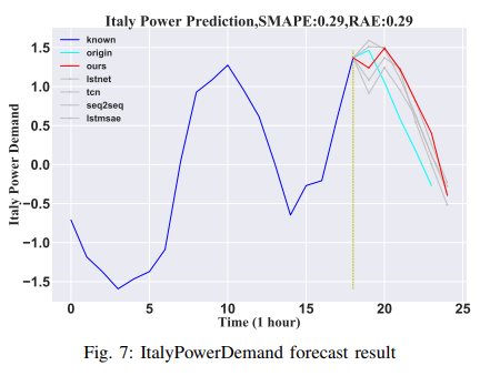
Electricity Demand in Italy
The dataset is derived from a 12-month time series of Italian electricity demand; 1029 samples were trained and 67 samples were evaluated. Each set has a total of 24 samples. In this experiment, the first 18 hours of data are used as input to predict the subsequent 6 hours of data. The results are shown in Fig. 7.
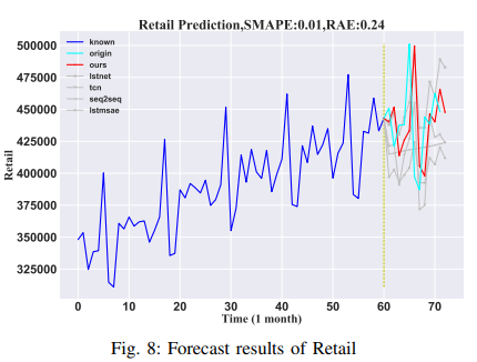
Retail
The Kaggle dataset provides monthly retail sales data for the United States from January 1, 1992, to May 1, 2016. There are a total of 293 samples. For this paper, 95% of the data was used as a training set and 5% as a test set. To predict the next 6 months of data, we used the last 12 months of data as input. The results are shown in Fig. 8.
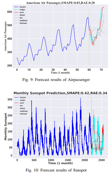
Airline Passenger
This data set provides monthly passenger counts for American Airlines' foreign carriers from 1949 to 1960. The total sample size is 144. The training set consists of data from 1949 to 1959, and the test set consists of data from 1960. The input data spans 60 months, with 12 months of forecasts. The results are shown in Fig. 9.
Sunspots
The dataset consists of monthly sunspot observations (1749-2019) and is 2820 samples; 95% were used as a training set and the last 5% as a test set. The input data is 2200 months long and predicts 360 months of future data. The results are shown in Fig. 10.
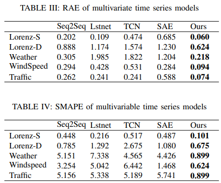
C. Multivariate time series
The results of the multivariate analysis of five representative data sets are shown in Table III and Table IV. The weather data set, the traffic data set, the wind speed data set from actual observations, and the two artificial Lorenz data sets are examples of multivariate data sets. These multivariate data sets are often typically chaotic systems and are more complex than univariate data sets, so it is necessary to add features to help with forecasting. To demonstrate this problem more effectively, Lorenz flalign (full-length align) created a Lorenz dataset that can be statistically adjusted for relevant parameters. Temperature, the target variable of the weather dataset, was a good choice to demonstrate the interpretability of the model since it has a variety of modal cycles and is influenced by several additional factors. Due to the very high uncertainty in the traffic and wind data sets, it is necessary to employ known future factors to aid in forecastings, such as wind speeds and average vehicle speeds from other stations. Other models also include known future elements, but the results are poor, demonstrating that the models in this study have a strong understanding of the characteristics of spatial information.
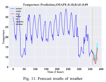
Weather Forecast
Datasets spanning 2006-2016 were obtained from Kaggle. Temperature predictions for this experiment depend on other variables such as humidity, wind speed, wind direction, visibility, cloud cover, and barometric pressure. The data contained a total of 96453 samples split by time. Ninety-five percent of the data was used for training and 5% for testing. The model used the data from the first 2200 hours to predict the temperature for the next 360 hours with external features. The results are shown in Fig. 11.
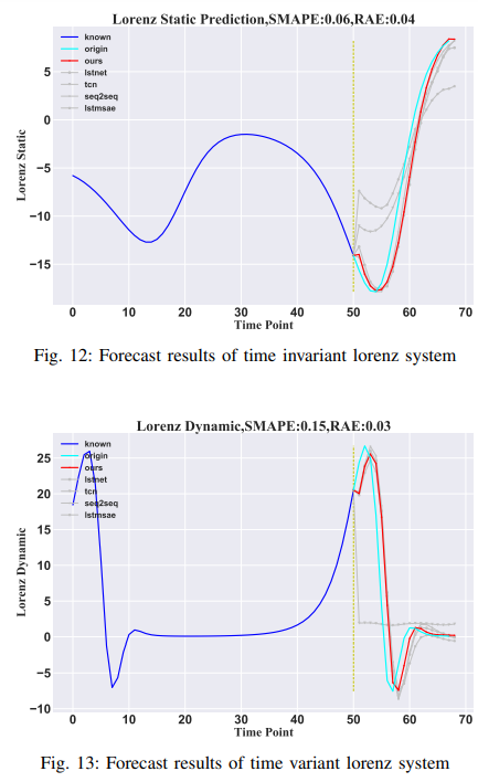
Lorenz
where G(-) is the Lorenzian nonlinear function set of X(t) = (xt1, . . . , xt90)′ of the Lorenzian nonlinear function set and P is the parameter vector. In this paper, the time-invariant and time-invariant Lorenz systems are tested to show the distinction between the models described by the time-invariant and time-invariant systems, respectively. In the time-invariant Lorenz system (Lorenz-S), P does not vary over time, while in the time-varying system (Lorenz-D), P does. In the experimental simulations, 5000 samples were generated, with the first 90% of the data used as the training set and the last 10% as the test set. The experimental results show that the model presented in this paper works well for both time-varying and time-invariant systems. The results are shown in Fig. 12 and Fig. 13.
Wind speed
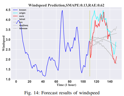
This dataset is high-dimensional (155-dimensional) wind speed data from 155 stations in Wakkanai provided by the Japan Meteorological Agency, recorded every 10 minutes for a total of 138,600 minutes. In this paper, the known duration of 110 minutes is used to estimate wind speeds for the subsequent 40 minutes. Data from the other 154 sites were used as an additional feature, and the target wind speed for one of the 155 sites was chosen at random. Predicting wind speed is considered to be very difficult, but this method provides very good wind speed prediction results. Predicting wind speed is considered very difficult, but this method predicts better results than other methods. The results are shown in Fig. 14.
Traffic volume
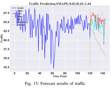
Average vehicle speed (MPH) is predicted using data from 207 loop detectors along Route 134 in Los Angeles, with each detector observation treated as a separate variable. The first 120 hours are used to predict the average speed over 24 hours. From the high-dimensional data, data from one sensor is chosen as the target variable, while observations from other sensors are used as auxiliary features. This demonstrates the model's ability to predict spatial data. The results are shown in Fig. 15.
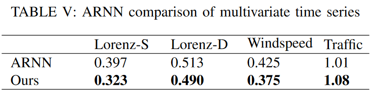
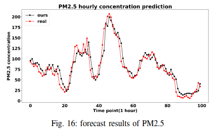
For a better comparison, instead of reproducing the paper, we followed the experimental results of ARNN (Automatic Reserve Pool Neural Network) and tested it on the Lorenz, wind speed, and traffic datasets, using RMSE as the metric. The results are shown in Table V. To show that TSDFNet performs well on the single-step forecasting problem, we compare it to LSTM-SAE on the air quality dataset. The forecast covers PM2.5 concentrations from 2010 to 2014, and the model achieves a significant reduction in RMSE (from 24 to 15). The results are shown in Fig. 16.
D. Discussion
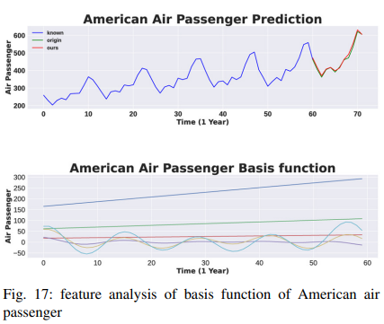
After establishing the performance advantages of TSDFNet, we show that this model design allows us to analyze its specific components to explain the general relationships learned by the model. First, we quantify the importance of the features by analyzing interpretable variants of the TDN described by equation (4). The air passenger data set is not stationary and contains a mixture of seasonality and trends. This increases from year to year and changes frequently from month to month. The results are shown in Fig. 17, where the original signal and its prediction are displayed in the top row of the figure and the basis functions in the second row.
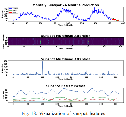
The results for the sunspot data set are shown in Fig. 18. The top row of the figure shows how seasonality is present, while the bottom row shows how well the periodicity was captured by the fine-tuned trigonometric basis functions. In addition, the attention weight patterns that TSDFNet uses to highlight decisive moments based on inferences may also be quite informative: in the second row, you can see many bright stripes spaced out against a dark background. These represent the start of a new cycle; aggregating the selection weights for each time step, as shown in the third line, we see that the spikes of interest coincide with the sunspot troughs.
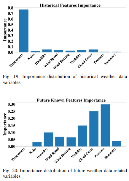
Furthermore, the importance of each feature, as determined by (11), can be examined using the decision weight pattern of the feature selection block. The important distribution of historical features is shown in Fig. 19, while also considering other feature components of historical data. It can be seen that the historical temperature data accounts for about 75% of the importance of future temperature data. The important distribution of future known data is depicted in Fig. 20. It can be seen that the accuracy of the forecast is highly dependent on the future pressure and cloud thickness. Also, future temperature data is not known and is filled with a value of 0, so its contribution to the results is zero. We also use Gaussian noise as input to show how our model can eliminate unimportant variables. The contribution of Gaussian noise is minimal because it has no relevant information.
summary
This paper introduced the Temporal Spatial Decomposition Fusion Network (TSDFNet), a new interpretable deep learning model that incorporates feature engineering into modeling and achieves phenomenal performance.TSDFNet is a new model that uses utilizes special components to handle the long-term prediction problem for time series: the Temporal Decomposition Network (TDN) can be customized with any basis function as an eigenmode for time series decomposition; the Spatial Decomposition Network (SDN) uses external features as basis functions for sequence decomposition; the Adentive Feature Fusion Network (AFFN) fuses all input features and selects the most important ones; and the Spatial Decomposition Network (SDN) uses the most important features as basis functions for time series decomposition. Finally, extensive experiments have demonstrated that TSDFNet consistently yields state-of-the-art performance compared to various well-known algorithms.


Categories related to this article


