Low Cost & High Accuracy! Reservoir Computing Model For Capturing Multiscale Temporal Features
3 main points
✔️ An extension of Echo state network, an effective low-cost method for time series forecasting
✔️ Uses multiple independent reservoirs to model multi-scale time features
✔️ Successful high accuracy in benchmark and real factory power load forecasting
Long-Short Term Echo State Network for Time Series Prediction
written by Kaihong Zheng, Bin Qian, Sen Li, Yong Xiao, Wanqing Zhuang, Qianli Ma
(Received May 2, 2020, accepted May 9, 2020, date of publication May 14, 2020, date of current version May 28, 2020)
Comments: Published in IEEE Access.
The images used in this article are from the paper, the introductory slides, or were created based on them.
first of all
This paper introduces a new type of low-cost and high-efficiency time series task model Echo State Network ( hereafter ESN) which has attracted attention as a low-cost and high-efficiency time-series task model.
In the last few years, time series analysis has become a very active research field. In particular, time series forecasting has been applied to a wide range of fields such as agriculture, commerce, meteorology, and medicine. Time series forecasting is based on feed-forward networks (FFN) and Support Vector Regression (SVR) and Recurrent Neural Network (RNN) and many other methods. Among them RNN is a recurrent neural network ( recursive ) RNNs can approximate arbitrary nonlinear systems with arbitrary accuracy due to recurrent connections between neurons, making them excellent for handling complex nonlinear time series data.
However RNN is a BPTT algorithm, RNNs suffer from slow learning convergence, high computational cost, gradient vanishing/explosion, and local optimal solutions. To solve these problems, an efficient recurrent network model called ESN was proposed as an efficient recurrent network model to solve these problems. And the proposed method in this paper is based on this ESN without compromising its efficiency, and it can predict more complex time series data with high accuracy. We will introduce the innovations and their effects.
Echo State Network What is
Before explaining the proposed method, we will discuss the usual ESN We briefly introduce The time-series information is stored in a reservoir (reservoir) and the echo (echo) The network is updated so that ESN is composed of three layers: input layer, reservoir layer and output layer as shown in the figure below. three layers as shown in the figure below. ESN The most important feature of The weights to be learned are the output layer weights $W_{out}$ only in the ESN. The other input layer weights $W_{in}$ and the reservoir layer weights $W_{res}$ are randomly initialized before learning and fixed at their values. Therefore, the conventional RNN can obtain an optimal global solution by preventing gradient vanishing and explosion without taking time for convergence and training.
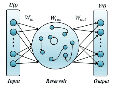
Here is the updated formula for the network.
$x(t)=\gamma \cdot \tanh (W_{in} u(t) + W_{res} x(t-1))+(1-\gamma)\cdot x(t-1)$
$y(t)=W_{out}x(t)$
where $u(t)$ is the input, and $x(t)$ is the reservoir state, and $y(t)$ is the output. is the output. $W_{in}$ , and $W_{res}$, $W_{res}$. , and $\gamma$ are hyperparameters that determine how much of the previous state is taken into account in the leakage rate. Only the output weights are learned by solving a linear regression problem. The output weights can be updated by a simple linear regression because the nonlinear, high-dimensional mapping in the reservoir layer captures the dynamics of the input.
ESN has shown excellent performance in time series forecasting, but it is difficult to model multiscale time features, i.e., complex time series data. This is because ESN has only a single recurrent module. Therefore ESN layers of DeepESN and MESM However, these methods tend to model long-term temporal features and ignore short-term features, and the size of the reservoir increases with the number of layers.
The proposed method (LS-ESNs)
ESN In contrast to the ESNs, the Long-Short term Echo State Networks (LS-ESNs) proposed in this paper are aimed at modeling more complex multi-scale temporal features. Long-Short term Echo State Networks (LS-ESNs) LS-ESNs. LS-ESNs are not stacked layers, but rather 3 Instead of stacking layers, LS-ESNs consist of three independent reservoirs with different recurrent connections as shown in the figure below. Each reservoir is a Long-term reservoir Typical reservoir Short-term reservoir and can capture the dependency of different time scales. In this section, we will explain the details of each network and the processing of the output layer.
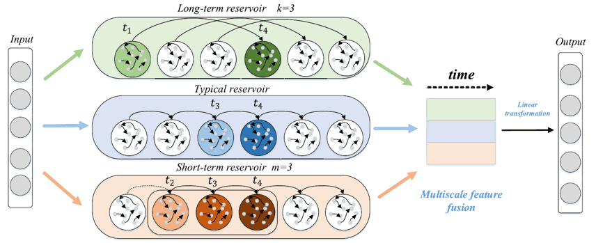
Long-term reservoir
Long-Term Reservoir is a reservoir specialized in capturing long-term features by skip connections. The update equation is the following equation
$x_{long}(t)=\gamma \cdot \tanh (W_{in}u(t)+W_{res}x_{long}(t-k))+(1-\gamma)\cdot x_{long}(t-k)$
where $k$ is the length of the step to be skipped and the larger the value, the longer the time scale to be considered and the more the reservoir state is updated depending on the information of the earlier time.
Typical reservoir
A typical reservoir is a typical ESN The update equation is the same as for the normal ESN.
$x_{typical}(t)=\gamma \cdot \tanh (W_{in}u(t)+W_{res}x_{typical}(t-1))+(1-\gamma)\cdot x_{typical}(t-1)$
Time $t$. is particularly useful for updating the state at time $(t-1)$ information affects the state update at time $t$ in particular.
Short-Term Reservoir
Short-Term Reservoir is a reservoir that specializes in capturing short-term dependencies.
$x_{short}(t)=\gamma \cdot \tanh (W_{in}u(t)+W_{res}x(t-1))+(1-\gamma)\cdot x(t-1)$
$x(t-1)=\gamma \cdot \tanh (W_{in}u(t-1)+W_{res}x(t-2))+(1-\gamma)\cdot x(t-2)$
︙
$x(t-m+1)=\gamma \cdot \tanh (W_{in}u(t-m+1)+W_{res}x(t-m))+(1-\gamma)\cdot x(t-m)$
Typical reservoir The main difference between $m$ is introduced. Typical reservoir introduces a time $t$ to the reservoir state at time 0 to time $(t-1)$ while all the information from time 0 to time $(t-1)$ is stored in the Short-Term Reservoir is $(t-1)$. to $(t-m+1)$. i.e. $m$. to $(t-m+1)$, that is, $m$. The actual process is to find the time $t$ to calculate the reservoir state at time $t$. $x(t-m)$ is reinitialized by a normal distribution and recomputed. By doing this, only the last $m$ of history information is taken into account.
Output Layer Processing
3 From the two reservoirs $x_{long}(t)$ , we have $x_{typical}(t)$, and , and $x_{short}(t)\in \mathbb{R}^{N\times 1}$ and then concatenate them to obtain the multiscale time representation $X(t)=[x_{long},x_{typical},x_{short}]$. and then concatenate them. Then we can use the usual ESN We calculate the output layer in the same way.
$y(t)=f_{out}(W_{out}X(t))$
experimental results
Experiment benchmarks two-time series forecasts Monthly Sunspot and Lorenz and real factory power load data.
predictive accuracy
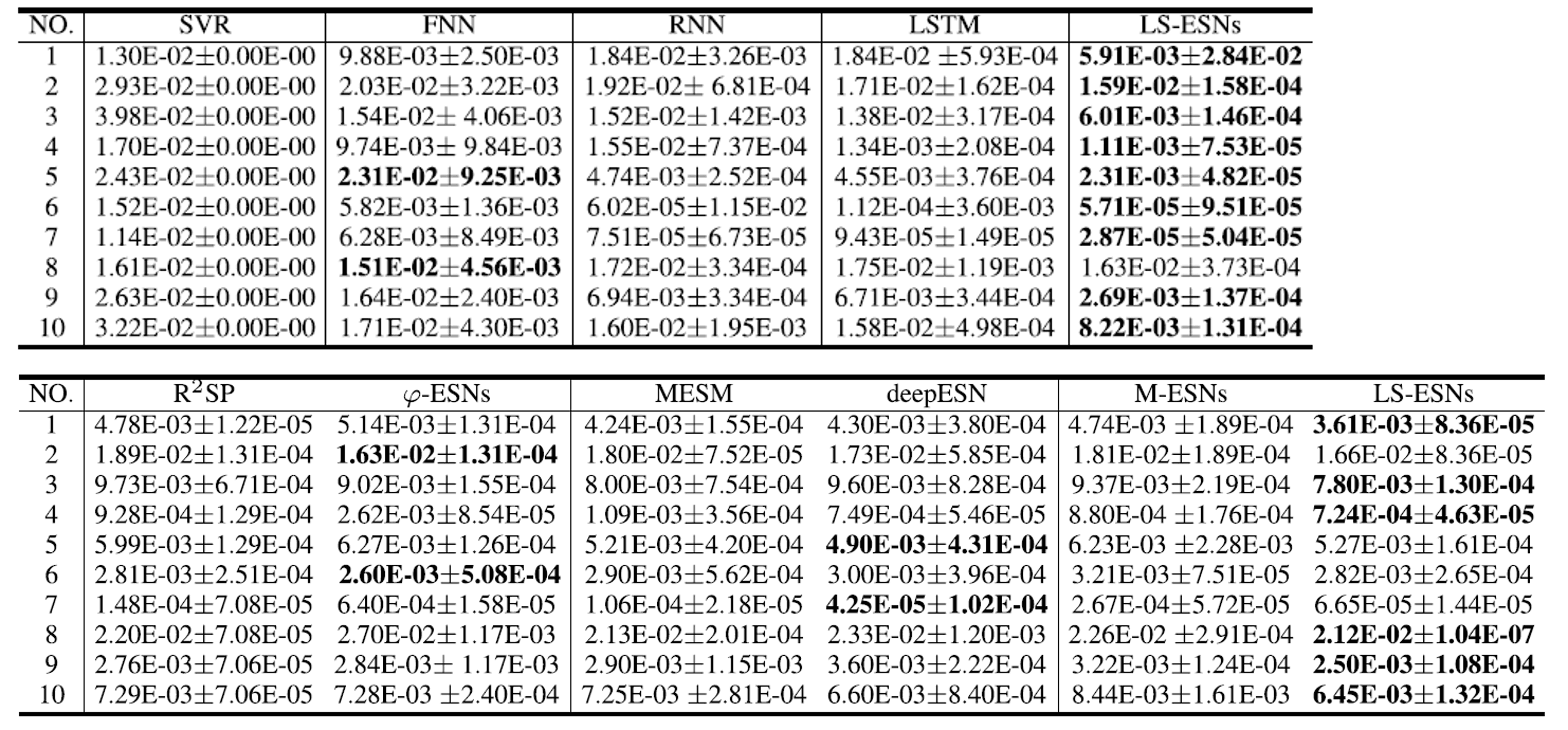
The evaluation indicators are MSE, the NRMSE and SMAPE MSE, NRMSE, and SMAPE. The comparison methods are the classical methods introduced in the beginning FNN, and SVR, and RNN and LSTM and ESN method based on $\varphi$- ESNs and R$^2$SP, M MESM, MESM DeepESN M-ESNs M-ESNs are M-ESNs are LS-ESNs of 3 All of 3 layers Typical reservoir method. First of all Monthly Sunspot and Lorenz, We will show the prediction results of
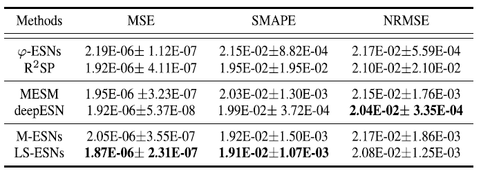
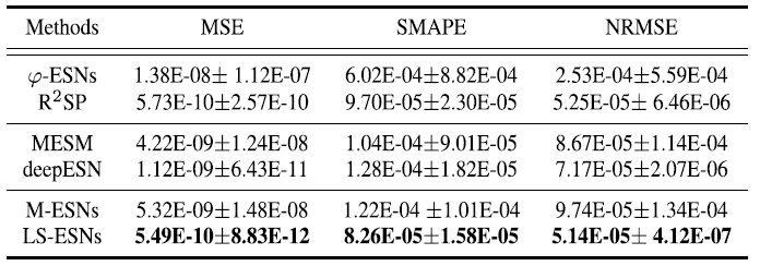
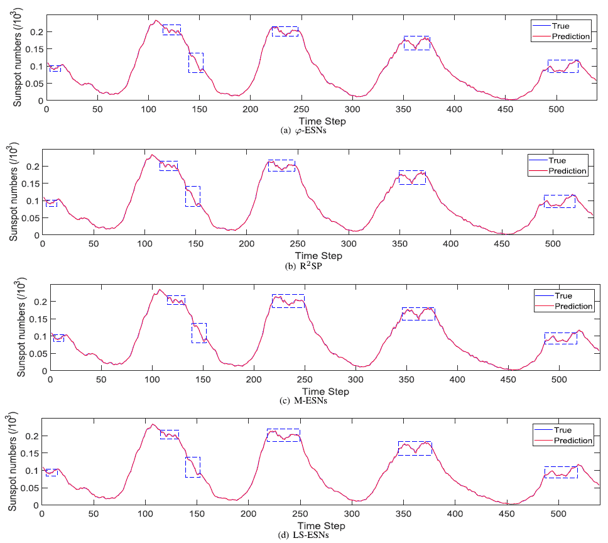
Monthly Sunspot of NRMSE Excluding 5 The proposed method recorded the best accuracy in all five metrics except NRMSE of Monthly Sunspot. FNN and SVR were excluded because of their low prediction accuracy. In addition, comparing the actual prediction results (shown below), the ESN-derived methods were able to predict, but LS-ESNs are better at predicting the non-smooth and complex regions outlined in blue. This shows that capturing multiscale temporal features improves the prediction performance for complex local patterns.
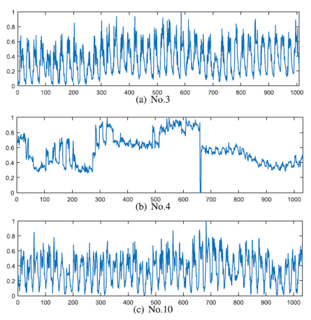
As for the power load prediction of actual factories, the error was minimized for most of the indicators. Because of the large number of data, this article will focus on MSE results are shown below. This data is No.1~No.10 and each of them has a different trend as shown in the figure below. It can be said that the advantage of the multi-scale feature is that the error can be minimized for each data group with such different behaviors.
Analysis of memory capacity
Here is a list of LS-ESNs s memory capacity. The data we use are univariate time series uniformly sampled from each time step [-0.8,0.8]. The task is then to reconstruct the signal. Each time step target value is expressed as $y_k(t)=u(t-k)$. For the sake of comparison MC score (memory capacity score) for comparison, and evaluate how well it reflects the input time-series information.
$MC=\displaystyle \sum_{k=0}^{\infty}r^2 (u(t-k),y_k(t))$
where $r^2(u(t-k),y_k(t))$ is the squared correlation coefficient between the input $u(t-k)$ and the reconstructed value $y_k(t)$ for delay $k$.
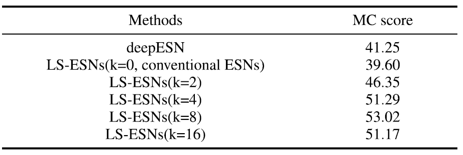
The results are shown in the figure above. The LS-ESNs obtained higher MC scores than the deepESNs of existing studies and the model using conventional ESNs. In particular, the LS-ESNs with $k=8$, which recorded the highest value, showed about 30% improvement over the existing studies.
Ablation study
Long-term reservoir and Short-term reservoir We eliminated one or both of them and compared the models to confirm the effect of From the power load forecast data Two from the power load forecasting data were randomly used.
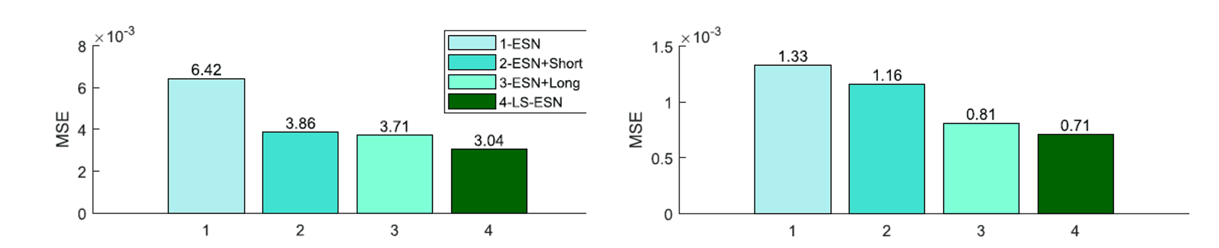
As a result, the best results were obtained by including both models, and the accuracy was improved by using only one model. In addition, the Short-term reservoir rather than Long-term reservoir The importance of the long-term characteristics is clear.
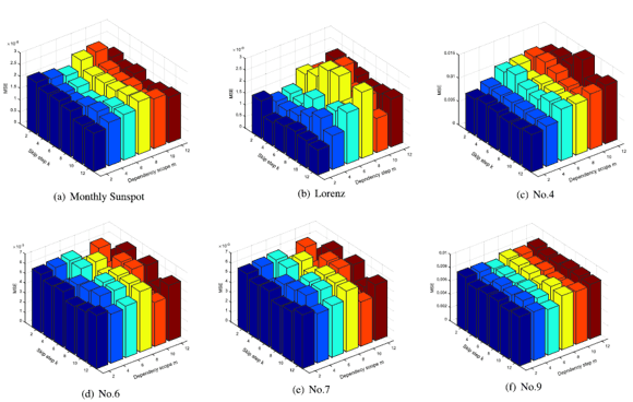
Impact of hyperparameters
LS-ESNs In Long-term reservoir Skip a step in $k$ In the Short-term reservoir the short-term dependence range $m$ in the short-term reservoir. First of all For $k$ for By increasing the value of $k$ we can capture the long-term dependence. However, if the value of $k$ is too large, it ignores a lot of information, and if it is too small, it cannot capture the long-term periodicity. Therefore, it is better to use $k$ which is suitable for the characteristics of the data. This is shown in the following figure (a) of the Monthly Sunspot result in (a) below. Because the periodicity of this data set $k$ increases the value of MSE value also improves. Next, we need to find the value of $m$ is set small in the case of the data set which contains violent fluctuation without periodicity, the value of MSE improvement was observed. In the figure below (c)No. 4 (c) No. 4 in the figure below is the data of power load forecast of a factory, which has no periodicity as shown in the above figure. It was shown that the modeling of short-term characteristics is effective for this kind of data.
summary
In this article, we introduced LS-ESNs as an effective method for capturing multiscale temporal features. The model is characterized by the use of three independent reservoirs with different recurrent connections. Experiments showed the effectiveness of LS-ESNs by using benchmark time series forecasts and real power load data. We also discussed the effect of each reservoir newly introduced in this method and the effect of hyperparameters.
As a prospect, it is required to model and predict the dependency among variables in multivariate time series, because it corresponds only to univariate time series at present. I look forward to the further development of reservoir computing!


Categories related to this article


