RCURRENCY, A New Possibility For Stock Prediction
3 main points
✔️ Proposed an RNN-based stock prediction model
✔️ Adds LSTM layer to enhance versatility for time series
✔️ Useful for a variety of digital assets
RCURRENCY: Live Digital Asset Trading Using a Recurrent Neural Network-based Forecasting System
written by Yapeng Jasper Hu, Ralph van Gurp, Ashay Somai, Hugo Kooijman, Jan S. Rellermeyer
(Submitted on 13 Jun 2021)
Comments: Published on arxiv.
Subjects: Artificial Intelligence (cs.AI)
code:
The images used in this article are either from the paper or created based on it.
First of all
Since the advent of modern financial markets in the 17th century, experts have have used the term Commodities , and Services stocks Stocks The company has Various efforts have been made to maximize the profits derived from the trading of securities. Over the past few decades, several studies have been conducted on the potential of artificial intelligence in trading stocks in the traditional market, with some success.
Additionally, modern machine learning algorithms can discover patterns in data that are invisible to the human eye due to the volume and complexity of the data.
In this article, I will summarize the paper "RCURRENCY: Live Digital Asset Trading Using a Recurrent Neural Network-based Forecasting System", which I will summarize.
Related work
Using historical data to predict stock prices has been an active research topic for decades.
The early methods used a purely analytical approach, applying basic mathematics and statistics, but since that time there have been several approaches to predicting stock prices and how good or bad the results should be.
For example, if the random walk strategy accurately reflects reality, then empirical evidence shows that all models on (stock) market forecasting are meaningless. Recently, more and more variables have been added to forecasting models, such as market volume, Twitter sentiment, investor sentiment, and media news content.
Whereas fundamental analysis describes the examination of data with a focus on macroeconomic variables, technical analysis focuses on extracting trends and patterns in the price, volume, breadth, and trading activity of an investment instrument.
The methods proposed and analyzed in this paper focus on technical analysis, but we also intend to address fundamental analysis in the future.
Random Walk... A hypothesis that the price movements of a financial instrument have no regularity and are in no way related to past fluctuations. See below for details.
Fundamental analysis... A method of analysis that predicts medium- to long-term movements in foreign exchange markets based on information on the world economy, economic indicators of each country, and political trends.
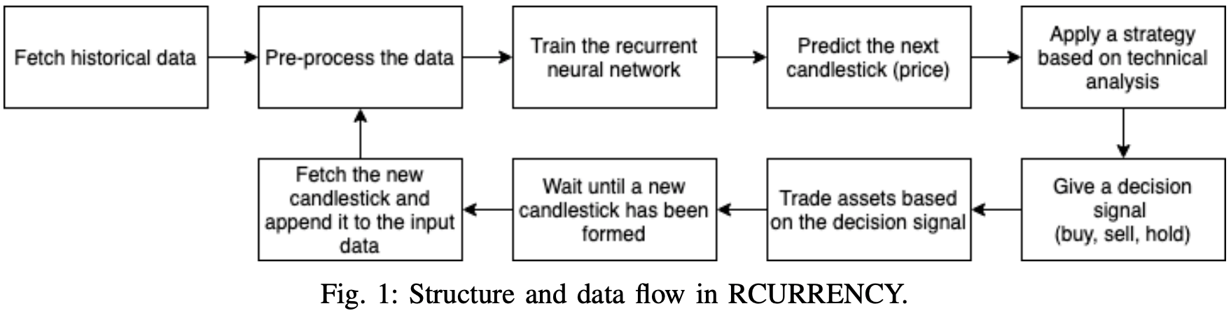
RCURRENCY live trading system
In order to make reliable forecasts of the cryptocurrency market, the model we will use is the RCURRENCY system, which consists of three independent components.
The role of the first component is to collect and pre-process a set of timely aligned data.
The second component feeds this data into a neural network that is trained to recognize patterns in the processed data. These two components give the system the ability to predict single steps in time series data.
The third component is the ability to make single forecasts as well as trading decisions.
One can make trading decisions based on a precise analysis of trends and patterns, not only based on a single prediction, but also on a precise analysis of trends. This component contains a variety of trading strategies that calculate buy and sell signals based on their respective forecasts, each of which calculates buy and sell signals based on predefined rules. The flow diagram of the RCURRENCY system with all of the above components is shown below.
learning data
This system obtains raw Bitcoin training data by calling the API provided by CryptoCompare. CryptoCompare provides services on more than 3,000 digital assets and has the capability to retrieve historical price data.
Such data consists of candlesticks (four price movements of the opening price (OPEN), high price (HIGH), low price (LOW), and closing price (CLOSE) along a time series) data points for a one-minute time frame.
The raw data is subjected to preprocessing. Unfortunately, the first 30% of the data set contains many values that are close to zero, which tends to reduce the predictive power of the network. This can reduce the predictive ability of the network. These values do not contain enough variance to allow the gradient descent of the error function to converge. As a result, we have manually removed all data up to May 2013.
Next, technical analysis is performed to extract trends and patterns from the price data and to create technical indicators. Each indicator is calculated according to its own formula, and each formula uses part or all of the data set as input.
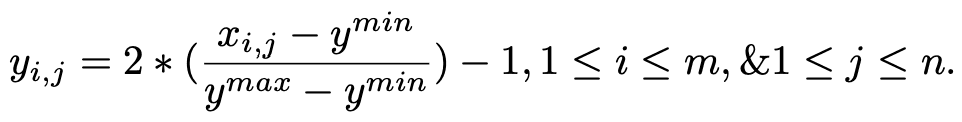
RCURRENCY implements financial technical indicators. The values of the calculated indicators are added to the training data. This additional training data allows the neural network to obtain more information about the market and higher prediction accuracy. Finally, a row-based normalization is applied to the dataset to make it fall in the range of -1~1. This gives good results and reduces the training time.
A new row normalized matrix is mathematically defined as follows Given a matrix x of dimension m × n , then For a new matrix y The following equation holds the following equation holds
recurrent neural network
We use a recurrent neural network as a predictor of RCURRENCY. A recurrent neural network is a type of neural network that can exhibit dynamic behavior over time.
The network models the connections between the nodes of a layer as a directed graph along a continuous time The input data of the RCURRENCY recurrent neural network consists of candlesticks. The values of the candlesticks depend on the values of the previous candlesticks, so it is not a random walk.
In traditional recurrent neural networks, gradient descent is a problem when learning long-time dependencies, but the use of LSTM layers in the architecture of recurrent neural networks solves the problem of gradient explosion and disappearance. The recurrent neural network consists of three layers.
1)Linear layer
The linear layer is necessary to make the nodes in the input layer correspond to the number of nodes in the hidden layer. The linear layer isafully connected layer where every edge has an individual weight. Fully connected layer.
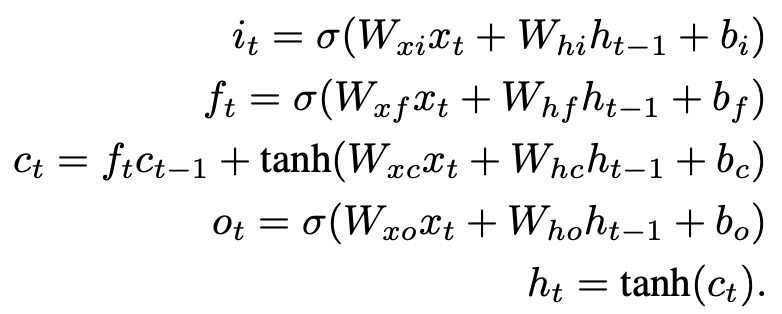
2) Fast LSTM layer
The FastLSTM layer is a special faster version of the conventional LSTM layer. The FastLSTM layer is aspecial, faster version of the conventional LSTM layer. The fast LSTM layer is a faster version of the traditional LSTM layer. input, forget and output gates,and hidden state computation in a single step. Since we are implementing the FastLSTM layer instead of the traditional LSTM layer,the synthesis function has been slightly modified.
Click here for more information about Fast LSTM layer
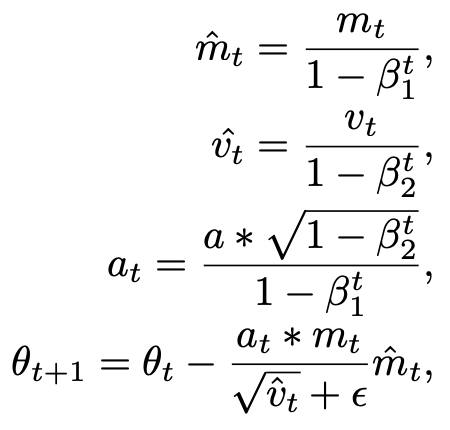
3) Output layer with Mean Squared Error (MSE) performance function
The output layer evaluates the neural network when it is used for learning purposes. The MSE function is used to evaluate the network.
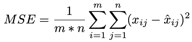
xij is the actual value, xˆij is the predicted value in row i and column j
predicted values in row i and column j, m is the total number of rows
n is the total number of columns
The expression to update the parameters is
Trading Strategies and Forecasts
There is a long-standing discourse about how useful trading strategies actually are.
Common trading strategies based on time-series pattern analysis, such as momentum and contrarian, as well as other technical analysis strategies, have been used with varying degrees of success. Therefore, we added this element to our experimental AI ,. decided to make it possible to apply four different trading strategies based on technical indicators. A brief description of each trading strategy is given below.
Momentum: An expression used to describe the momentum of a market.
A contrarian is an investor who makes a market move in the opposite direction of the market trend. It is also referred to as a contrarian investor.
Rate of Change (ROC)
The ROC strategy considers the change in the predicted value relative to the last actual value.
It considers the relative change between the forecasted value and the most recent actual value. If that change falls below the lower and upper thresholds, or exceeds the middle or upper limit, it decides whether to sell, buy, or hold.
Relative Strength Index (RSI)
It identifies the upward or downward trend in property values. If the value of the RSI changes long enough, it is considered overbought (should be sold).
Double Exponential Moving Average (DEMA)
DEMA is a strategy that uses two moving averages to determine when to buy, hold, or sell an asset. When the two moving averages cross over, momentum shifts between long-term and short-term asset values, making it time to buy and sell.
Moving Average Convergence/Divergence (MACD)
MACD is a well-known strategy based on the difference between two moving averages of different lengths, called the slow moving average and the fast moving average. This difference is then compared to a moving average called the signal line. When the difference exceeds the signal line, a buy, hold, or sell decision is made.
random walk
A controversial but widely-valued investment theory known as the efficient market hypothesis states that there is no consistently profitable trading strategy because all available information is immediately reflected in asset values.
implementation
RCURRENCY is implemented in C++, with a variety of libraries at its core. First, historical data is obtained using the API provided by CryptoCompare. The live data is fetched in real time by creating a WebSocket connection with the exchange (Binance) and fetching it after the candle is formed.
After the historical data is acquired, it is preprocessed and provided to the neural network. In this process, we use two libraries, Armadillo and TA-Lib.
The Armadillo library has the highly optimized matrix calculation capabilities needed to manipulate regular data sets, while TA-Lib has the functionality needed to efficiently calculate technical indicators from stock market data.
The recurrent neural network is implemented using MLPack, which is a set of . A fast and flexible C++ machine learning library MLPack is a fast and flexible C++ machine learning library that provides a wide range of It implements a wide variety of configurable neural networks and machine learning methods.
experimental evaluation
Given the time-dependent nature of the data, we applied time-series k-fold cross-validation. The training dataset is divided into a training part consisting of p samples (80%) and a validation part consisting of q samples (20%), where each sample represents a single time unit value. The k represents the number of samples used in the validation step, or how many time units are predicted in each cycle of training and evaluation.
Next, to facilitate this validation method, we continuously train the model on samples 1, . , p, to generate a prediction for the next time p + 1, and then validate the prediction using the validation sample p + 1 and Sample 1, ... , p + 1.
Setting the value of k to 1 means that q cycles are performed to complete a series of cross-validation; increasing the value of k decreases the number of learning and validation cycles. After each cycle, the error is computed and stored. Finally, the error function is used to measure the performance.
Figure 2 shows the root mean square error for the selected number of folds, a range of values of k were tested to obtain the smallest error.
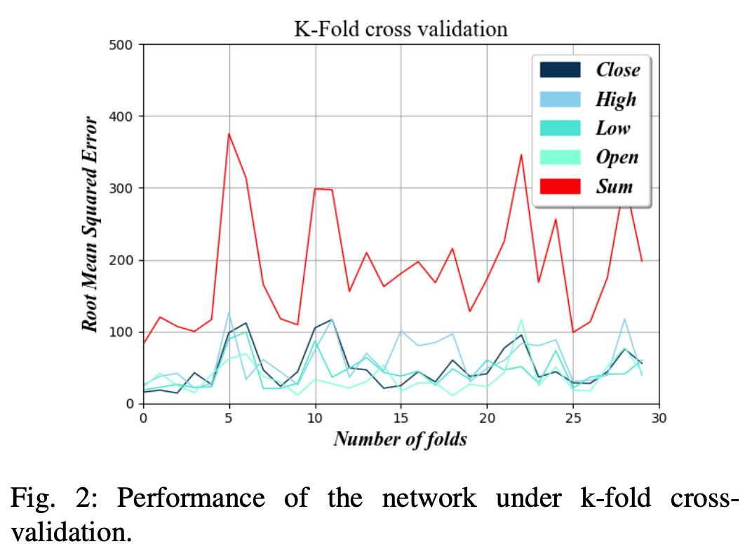
The lower the value of k, the less prediction error the AI will make. This is because the higher the number of folds, the less data is used to train the network before the prediction cycle.
We can also see that the prediction error for the four factors of opening price (OPEN), high price (HIGH), low price (LOW), and close price (CLOSE) is much lower than $50 for lower values of k.
This means that the system can accurately predict uptrends and downtrends because the absolute change in each interval is, on average, greater than the forecast error.
Parameter optimization
In order to optimize the hyperparameters, we applied the validation method of the previous section and searched for the minimum RMSE while changing the parameters one by one.
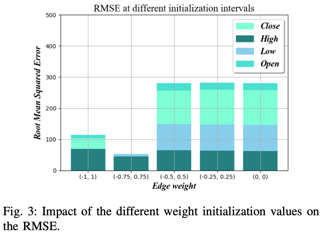
Initialization of edge weights
The initialization value of the edge has a significant impact on the training time of the neural network.
By setting the initial weights more optimally, the convergence of the final weight values is faster and the learning time can be significantly reduced.
As Figure 3 shows. , the -random numbers in the range of 0.75 and 0.75 proved to have the lowest RMSE in different folds of the bitcoin dataset.
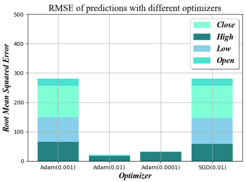
optimization algorithm
The role of the optimization algorithm is to adjust the weights at each training iteration of the network, affecting both the speed of convergence and the accuracy of the prediction.
The Stochastic Gradient Descent (SGD) method is the most commonly used optimization algorithm, and we tested it against the Adam optimizer with different step sizes and found that SGD has the best balance between speed and accuracy for a learning rate of 0.01. The results show that SGD has the best balance between speed and accuracy for a learning rate of 0.01.
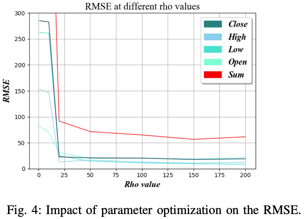
Rho value
Rho values are . Sets the length of the Back-Propagation Through Time (BPTT) used to train the network.
In practice, this determines how many recent values should be used to predict the output in the next step of the time series. As shown in Figure 4b, we find that the optimal value is about 150.
Complexity of hidden layers
The complexity of the hidden layer is the number of hidden nodes used in the FastLSTM layer.
Increasing the number of nodes has the potential to train more complex rules, but also increases the amount of data required for training. In addition, there is an increased risk of overfitting and loss of generalizability, which can lead to inaccurate results when the network is used with slightly different data sets.
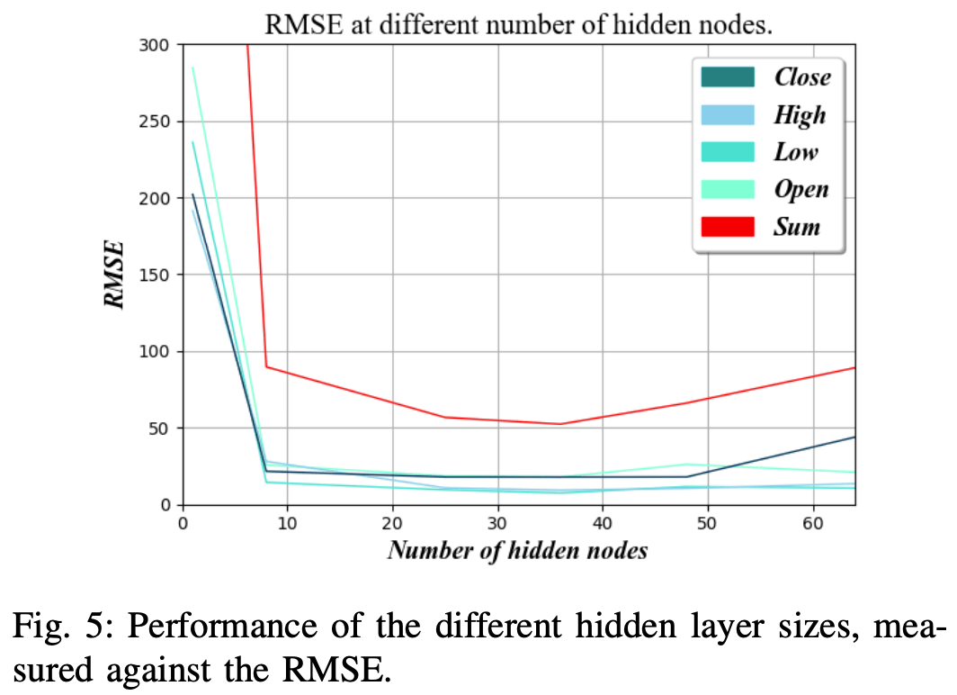
Figure 5 shows that the RMSE is the lowest when the number of nodes in the hidden layer is about 36.
Evaluating the results of trading strategies
In this section, we describe the trading engine and the results of our validation using historical data for each of the five trading strategies we have discussed.
The historical data serves as a simulation of the live inputs and updates the portfolio by executing hypothetical trades. The performance of each trading strategy in minimizing portfolio losses depends not only on the quality of the strategy itself, but also on the quality of the forecasts used to determine the course of action.
The recurrent neural networks in these experiments utilize the optimized parameter settings as described in the previous section to maximize prediction accuracy.
Each experiment covers the trading of a BTC/USDT pair, with BTC as the base currency and USDT as the quoted currency. The total value is calculated by converting the portfolio into the quoted currency each period. However, achieving a higher monetary value alone does not mean successful trading if the trader outperforms the market itself. If the value of BTC/USDT had continued to rise over a certain period of time, then the trader would have made a profit without having to do anything. This is a strategy called "Buy-And-Hold". In this strategy, you simply buy and hold a specified amount of an asset and do not trade any further. This strategy is an appropriate basis for comparison, in the sense that it "compares with Alpha". The results of this comparison and the experiment are shown in Figure 6.
BTC...Bitcoin
USDT... Stablecoins issued by Tether
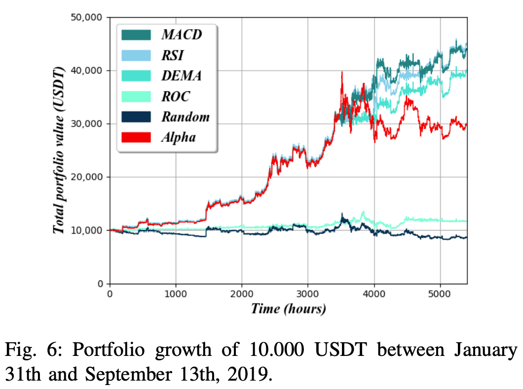
The AI is trained on about 90% of the data set , and used to predict the remaining 10% of the data. Each strategy was tested independently and each received an initial portfolio containing 10.000 USDT, which was then used to trade using approximately 5.400 hours of stock market data from January 31 to September 13, 2019. An alpha baseline was generated by simply converting 10.000 USDT to BTC at t = 0 and no further trading activity.
In order to achieve more stable results, some restrictions have been imposed on trading agents. Primarily, they can only trade up to 25% of their total portfolio at any one time. Also. , the If the expected increase in value based on the volume of trades is less than the trading commission (set at 0.1%), no trade will be made.
Figure 6 shows that in historical data for Bitcoin, the RSI strategy achieved the highest portfolio value, with the MACD strategy a close second and the DEMA strategy performing slightly worse. However, all three strategies maintained stable portfolio values, catching up to and even surpassing Alpha's baseline, with the ROC strategy performing almost as well as Random Walk, both barely maintaining a third of Alpha's baseline value. situation.
AI can outperform Alpha's baseline in certain strategies, but it's questionable whether the gains are worth the risk.
One way to answer this question is to calculate the Sharpe ratio. This is the ratio of the risk-free asset compared to the ,. The Sharpe ratio is a measure of how much return an investor is compensated for risk. The Sharpe ratio is , the the rate of return on the asset considered minus the rate of return on the risk-free asset Sharpe ratio divided by the standard deviation of the return rates of the assets considered.
Figure 7 shows the monthly Sharpe ratios for each of the six trading strategies measured over the last seven (hypothetical) months of the backtesting period from February 13, 2019 to September 13, 2019. The rate of return R is calculated as the ratio of excess return to the start of each month. With respect to the determination of the risk-free rate of return Rf, monthly U.S. Treasury bills (T-Bills) were the appropriate risk-free asset because the portfolio is measured in U.S. dollars.
During the backtesting period, the risk-free rate for T-Bills was approximately 2%, as shown on the U.S. Treasury website. Taking these numbers into account, a Sharpe ratio of 1 or higher is generally considered a good investment, while a Sharpe ratio of 2 or higher is considered an excellent investment.
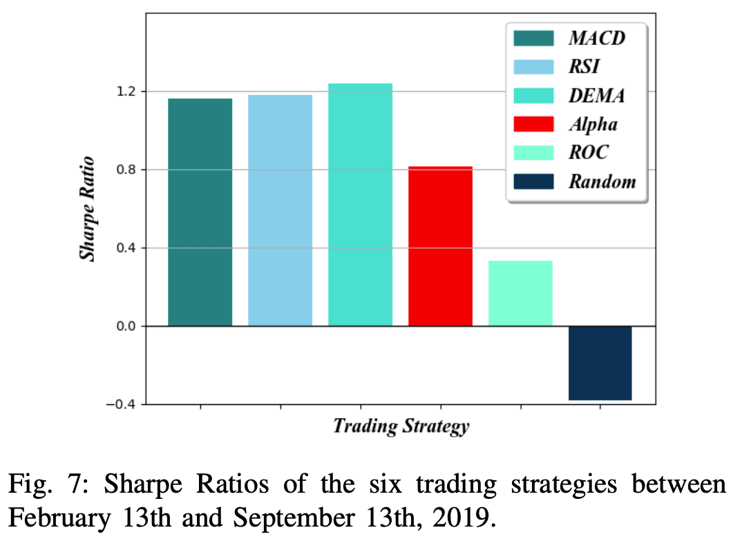
In this figure, we can see that the RSI and MACD strategies achieved the highest portfolio values, but the DEMA strategy maintained the highest Sharpe ratio. Since the returns (R) of the RSI and MACD strategies are high and the risk free rate (Rf) for each month is the same for all the strategies, we can assume that the RSI and MACD strategies have achieved the highest Sharpe ratio.
The Random Walk strategy suffered both large losses and high volatility, resulting in a Sharpe ratio below negative; the ROC strategy suffered similar losses but was able to maintain a positive Sharpe ratio due to the low level of volatility, while the ROC strategy suffered similar losses but was able to maintain a positive Sharpe ratio due to the low level of volatility. The ROC strategy suffered similar losses but was able to maintain a positive Sharpe ratio due to low levels of volatility.
summary
The TSKCV results suggest that the network is able to predict new asset values with an error of about 0.4% across the four output channels. Each strategy is successful in maintaining a stable portfolio value throughout the historical dataset at varying rates, but all strategies perform better than the randomized strategy.Even though RCURRENCY is tested on Bitcoin, its design can be adapted to other digital assets as well. Just none of the strategies could correctly predict a significant and sudden decline in asset value. However, this is a common problem with existing AI-based solutions, and future research could shed light on the question of whether more input data could improve their ability to effectively predict such events.


Categories related to this article
.JPG)